King profile validation - progenax — differentiable initial conditions for N-body simulations

The King suite verifies the lowered-isothermal Poisson ODE integration, the lowered-Maxwellian volume density (the 3-D density entering the Poisson source, distinct from the projected King K-function), and the matched velocity DF. Test file: tests/validation/test_king_physics.py (see the test dashboard for the live per-suite count); figures: scripts/validate_king.py.

What is verified¶

Each row maps to one or more assertions in test_king_physics.py. The Tolerance is the exact bound the test enforces; the Measured value is regenerated by scripts/validate_king.py (which prints an expected-vs-measured PASS/FAIL table for every figure).

Property	Tolerance (as tested)	Measured	Anchor
ODE boundary condition $\psi(0)=W_0$	$\|\psi(0)-W_0\| < 0.1$	0.0 (exact)	King’s dimensionless Poisson equation
Concentration $c=\log_{10}(r_t/r_c)$ , $W_0=2.5$ –15	$\le 0.03$ abs	max $\|\Delta\log_{10}c\| = 0.002$	King (1966) Table II
Volume density shape $\rho(r)$	$< 5\times10^{-3}$ max rel	$1.2\times10^{-10}$	oracle $\int_0^{\sqrt{2W}} v^2(e^{W-v^2/2}-1)\,dv$
Tidal truncation ( $r\le r_t$ )	100%	100%	self-consistent $r_t$ from $\psi\to 0$
Velocity boundedness ( $v\le v_{\rm esc}$ )	100%	100.00%	lowered-Maxwellian on $[0,v_{\rm esc}]$
Velocity isotropy $\langle v_x^2\rangle\!\approx\!\langle v_y^2\rangle\!\approx\!\langle v_z^2\rangle$	$< 10\%$ rel spread	$0.4\%$	isotropic DF
Dispersion profile $\sigma_{1d}(r)$	$< 12\%$ rel per bin	max rel $= 1.2\%$	analytic lowered-Maxwellian 2nd moment
Unscaled virial ratio $Q=T/\|V\|$	$\|Q-0.5\| < 0.05$	0.505 (no rescale)	$2T+V=0$
DF sampling differentiability ( $r_c, W_0, M$ )	AD $=$ central-FD	rel err $\le 2\times10^{-6}$	`jax.lax.scan` sampling, no `while_loop`

Figures¶

Generated by scripts/validate_king.py (prints expected-vs-measured PASS/FAIL for every panel). Each figure recomputes the same quantities the tests assert.

Concentration relation. progenax c=\log_{10}(r_t/r_c) (line) on King (1966)
Table II (open circles) across the full tabulated range W_0=2.5–15. Residuals
(panel b) stay within the \pm0.03 band — max |\Delta\log_{10}c| = 0.002.
W_0 \gtrsim 11 requires enlarging the ODE domain beyond the package default
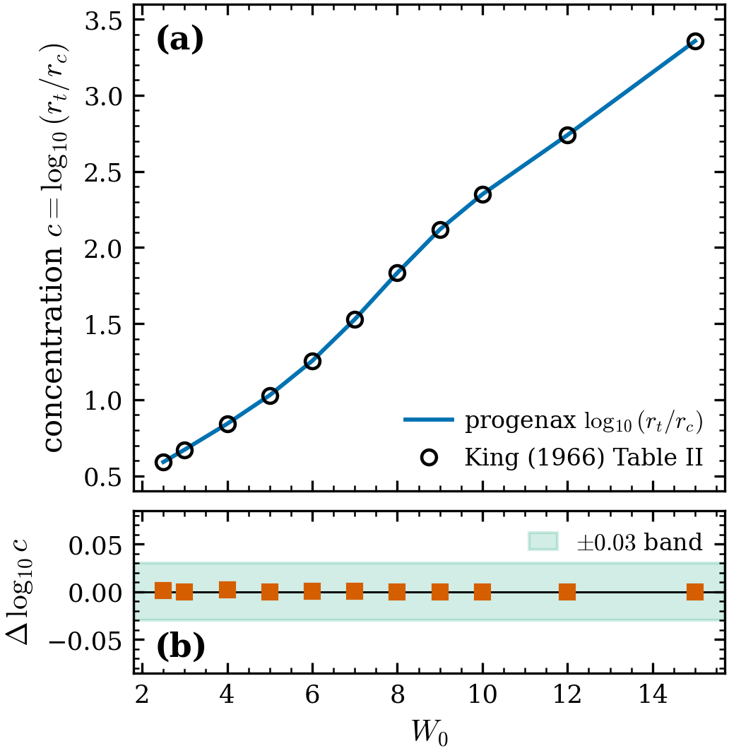
(see What this suite does not test); the figure does so per row. — Figure 1:**Concentration relation.** progenax $c=\log_{10}(r_t/r_c)$ (line) on King (1966) Table II (open circles) across the full tabulated range $W_0=2.5$ –15. Residuals (panel b) stay within the $\pm0.03$ band — **max $|\Delta\log_{10}c| = 0.002$** . $W_0 \gtrsim 11$ requires enlarging the ODE domain beyond the package default (see *What this suite does not test*); the figure does so per row.

Volume density vs an independent oracle (W_0=7). KingProfile.density
(dashed) coincides with the “King DF integral” — the direct velocity-space
integral \int_0^{\sqrt{2W}} v^2(e^{W-v^2/2}-1)\,dv of the defining DF, computed
independently (solid) — and with the N=5\times10^4 sample (points) to
max rel =1.2\times10^{-10} (panel b). This confirms the lowered-Maxwellian
volume density \hat\rho(W)=e^W\,\mathrm{erf}(\sqrt W)-\tfrac{2}{\sqrt\pi}\sqrt W\,(1+\tfrac23 W)
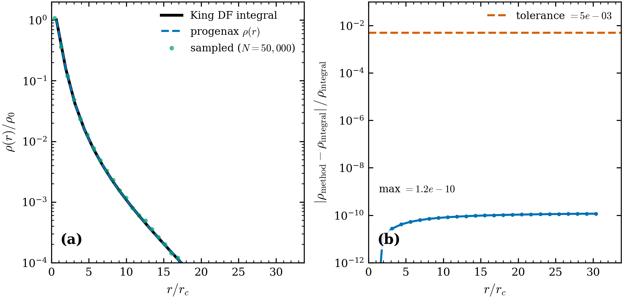
is the form used in the Poisson source. — Figure 2:**Volume density vs an independent oracle ( $W_0=7$ ).** `KingProfile.density` (dashed) coincides with the “King DF integral” — the direct velocity-space integral $\int_0^{\sqrt{2W}} v^2(e^{W-v^2/2}-1)\,dv$ of the defining DF, computed independently (solid) — and with the $N=5\times10^4$ sample (points) to **max rel $=1.2\times10^{-10}$** (panel b). This confirms the lowered-Maxwellian *volume* density $\hat\rho(W)=e^W\,\mathrm{erf}(\sqrt W)-\tfrac{2}{\sqrt\pi}\sqrt W\,(1+\tfrac23 W)$ is the form used in the Poisson source.

Velocity-space equilibrium (W_0=7). (a) Sampled \sigma_{1d}(r) on the
analytic King 2nd moment (per-bin rel \le 1.2\%). (b) Every velocity satisfies
v \le v_{\rm esc}(r) — 100% bound. (c) The unscaled IC sits at virial
Q=0.505: the matched lowered-Maxwellian DF is a true equilibrium with no
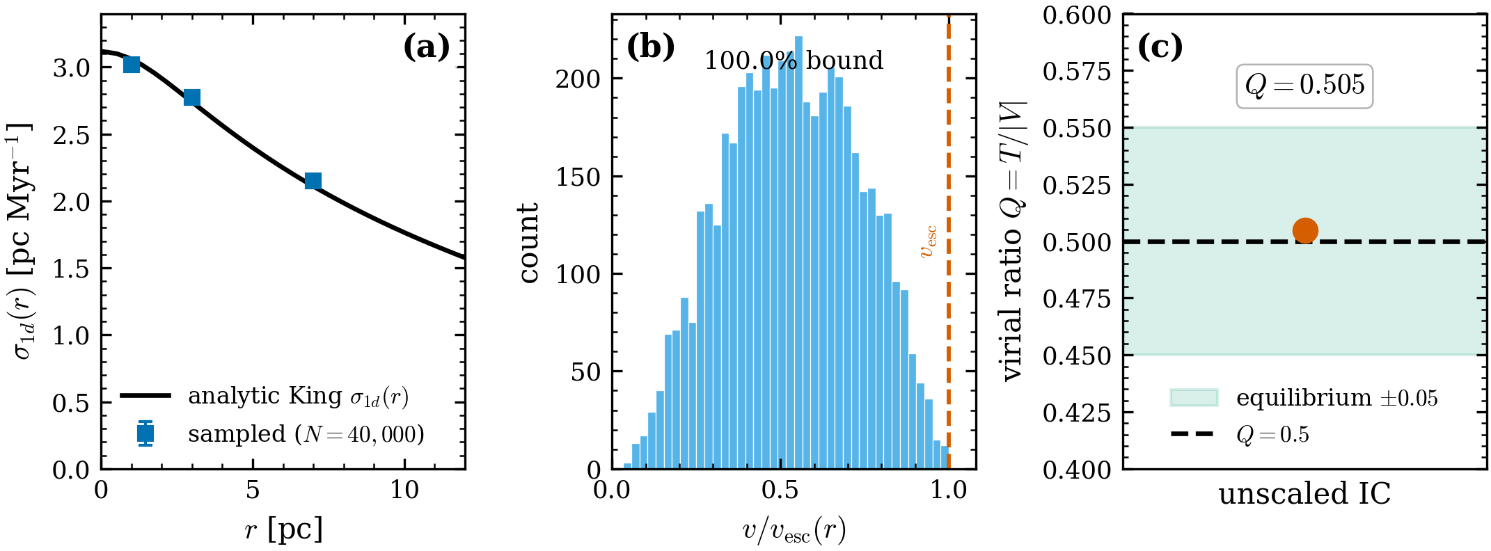
external rescale. — Figure 3:**Velocity-space equilibrium ( $W_0=7$ ).** (a) Sampled $\sigma_{1d}(r)$ on the analytic King 2nd moment (per-bin rel $\le 1.2\%$ ). (b) Every velocity satisfies $v \le v_{\rm esc}(r)$ — **100% bound**. (c) The unscaled IC sits at virial **$Q=0.505$** : the matched lowered-Maxwellian DF is a true equilibrium with **no external rescale**.

Table-routed speed draws vs the exact quadrature oracle (W_0=5,
N=2\times10^4). Since the 2026-06 memory batch, KingVelocityDF draws
speeds from a precomputed CDF table by default (SpeedCDFTable at g=1 —
the exact King reduction e^x-1 = E_\gamma(1,x), identity-test guarded); the
per-star quadrature is retained as speed_method="quadrature". The two
distributions are variate-paired and statistically indistinguishable (KS
D = 1\times10^{-4}, gate <0.02; moment ratios to <10^{-5}). Script:
scripts/validate_speed_routing.py; see
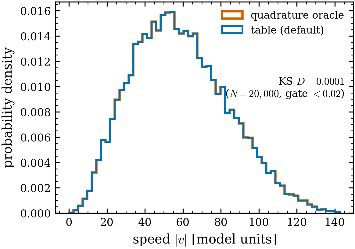
performance & memory. — Figure 4:**Table-routed speed draws vs the exact quadrature oracle ( $W_0=5$ , $N=2\times10^4$ ).** Since the 2026-06 memory batch, `KingVelocityDF` draws speeds from a precomputed CDF table by default (`SpeedCDFTable` at $g=1$ — the exact King reduction $e^x-1 = E_\gamma(1,x)$ , identity-test guarded); the per-star quadrature is retained as `speed_method="quadrature"`. The two distributions are variate-paired and statistically indistinguishable (KS $D = 1\times10^{-4}$ , gate $<0.02$ ; moment ratios to $<10^{-5}$ ). Script: `scripts/validate_speed_routing.py`; see performance & memory.

Concentration sweep. Normalized density for W_0=3,5,7,9; dotted lines and
floor markers give each model’s natural \xi_t=r_t/r_c, matching King (1966)
Table II (\Delta\log_{10}c \le 0.001). Higher W_0 ⇒ more extended, more
concentrated. from_W0_rc auto-sizes the ODE domain from W_0, so the full
tabulated range (to W_0=15, \xi_t\simeq2272) integrates without a manual
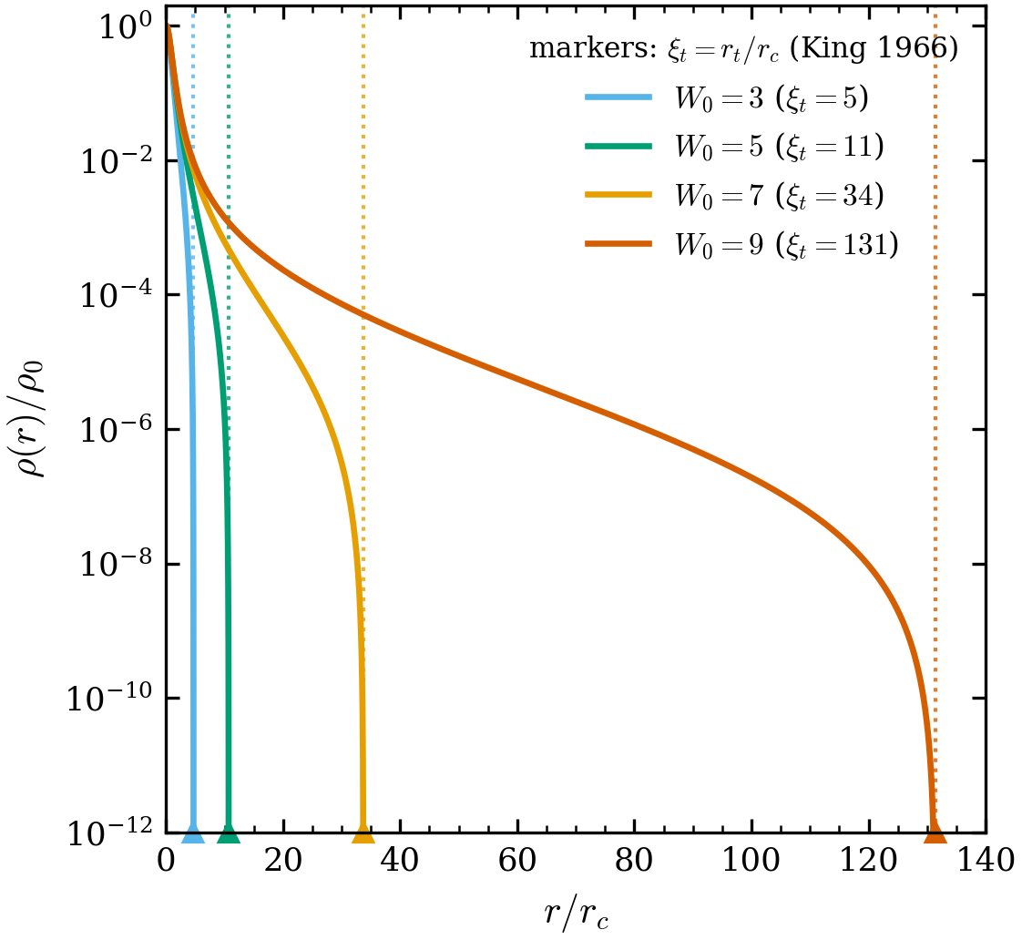
xi_max. — Figure 5:**Concentration sweep.** Normalized density for $W_0=3,5,7,9$ ; dotted lines and floor markers give each model’s natural $\xi_t=r_t/r_c$ , matching King (1966) Table II ( $\Delta\log_{10}c \le 0.001$ ). Higher $W_0$ ⇒ more extended, more concentrated. `from_W0_rc` auto-sizes the ODE domain from $W_0$ , so the full tabulated range (to $W_0=15$ , $\xi_t\simeq2272$ ) integrates without a manual `xi_max`.

Differentiability¶

The King IC pipeline is built for gradient-based inference: the model observables a likelihood uses — the density profile $\rho(r)$ and the velocity scale $\sigma_0$ — are differentiable w.r.t. the structural parameters that one fits to data.

Gradient validation (autodiff vs central finite difference). \partial(\text{observable})/\partial\theta
for each structural parameter \theta: (a) core radius r_c, (b) concentration
W_0, (c) total mass M_{\rm tot}. Autodiff (line) and finite difference (circles)
agree to max rel.\ err \le 2\times10^{-6} across the parameter range — so
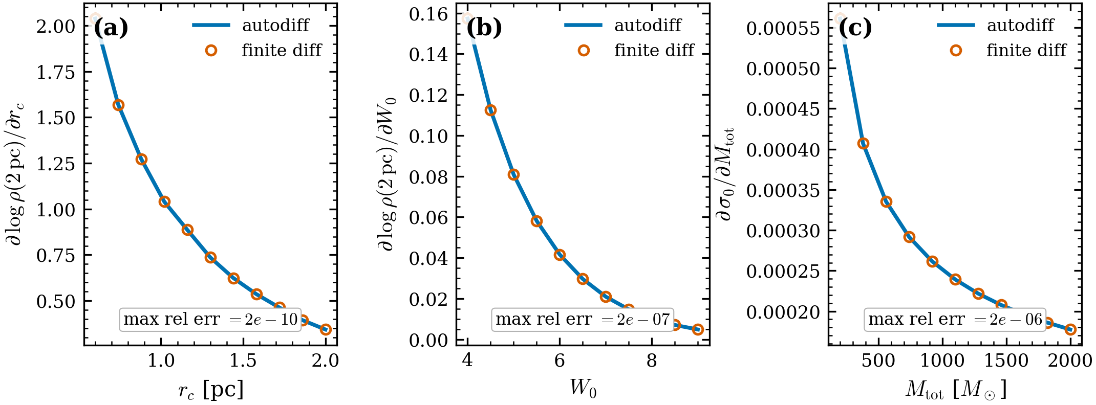
(r_c, W_0, M_{\rm tot}) can be inferred jointly by gradient descent or HMC. — Figure 6:**Gradient validation (autodiff vs central finite difference).** $\partial(\text{observable})/\partial\theta$ for each structural parameter $\theta$ : (a) core radius $r_c$ , (b) concentration $W_0$ , (c) total mass $M_{\rm tot}$ . Autodiff (line) and finite difference (circles) agree to **max rel.\ err $\le 2\times10^{-6}$** across the parameter range — so $(r_c, W_0, M_{\rm tot})$ can be inferred jointly by gradient descent or HMC.

What is differentiable in the King model.

Parameter	Differentiable?	Notes
$r_c$ (core radius)	✅ machine precision	The spatial scale; gradients flow through positions, density, and velocities.
$M_{\rm tot}$ (total mass)	✅ machine precision	Sets the velocity scale $\sigma_0\propto\sqrt{GM}$ .
$W_0$ (concentration)	✅ (profile observables)	Flows through the `diffrax` ODE → $\psi$ → density → CDF → sampling.
$r_t$ (scalar tidal radius)	✅ (zero-crossing slope)	$\partial r_t/\partial W_0$ is finite and exact — the unclamped $\psi=0$ crossing carries the implicit-function-theorem slope (the original silent-zero hazard was found and fixed by the gradient audit). Verified AD-vs-FD to $\sim 10^{-8}$ ( $\partial r_t/\partial W_0 \approx 22.9$ at $W_0=7$ , $r_c=1$ ).

The scalar

r_t

gradient is RESOLVED (differentiable)

KingProfile.from_W0_rc(W0, r_c).r_t now carries a finite, exact $\partial r_t/\partial W_0$ via the implicit function theorem, $\partial\xi_t/\partial W_0 = -\psi_{W_0}/\psi_{\xi}\big|_{\xi_t}$ (the source returns the unclamped $\psi_{\rm raw}$ , so the zero-crossing carries the slope). The forward value of $r_t$ is unchanged; only the gradient differs. This unlocks tidal-field coupling $r_t \approx r_J$ (inferring the Galactic potential / orbits from cluster limiting radii, wiring in progenax.tidal.jacobi_radius). The mechanism, the IFT design, and ranked science cases are at Differentiable King tidal radius ( $\partial r_t/\partial W_0$ ), which carries the full design record.

How to run¶

# physics tests (~30 s on CPU; ODE integration dominates)
pytest tests/validation/test_king_physics.py -v

# regenerate the five figures with PASS/FAIL tables
python scripts/validate_king.py

What this suite does not test¶

Multi-mass / anisotropic / rotating King — out of scope here. These are the generalizations formalized by Gieles & Zocchi (2015); progenax will implement them natively as its own differentiable lowered-model family (see the roadmap), rather than depending on an external package.

References¶

King (1966) is the original (Table II concentrations transcribed verbatim in the per-paper note). Theory and the factor-of-9 ODE derivation are at King profile; the lowered-Maxwellian DF at King velocity distribution functions.

References¶

King, I. R. (1966). The structure of star clusters. III. Some simple dynamical models. The Astronomical Journal, 71, 64–75. 10.1086/109857
Gieles, M., & Zocchi, A. (2015). A family of lowered isothermal models. Monthly Notices of the Royal Astronomical Society, 454, 576–592. 10.1093/mnras/stv1848