The Cartwright & Whitworth (2004) Q = m̄/s̄ parameter separates centrally
concentrated clusters () from fractal/substructured ones (). Test
file: tests/validation/test_substructure_q_physics.py (see the
test dashboard for the live per-suite count); figures:
scripts/validate_substructure_q.py.
What is verified¶
Each row maps to assertions in test_substructure_q_physics.py. Measured values
are regenerated by scripts/validate_substructure_q.py. The exact estimator uses the
CW04 area convention (convex-hull area biases high by ).
Property | Tolerance (as tested) | Measured | Anchor |
|---|---|---|---|
Uniform sphere (CW04 ‘3D0’) | 0.78 | Cartwright & Whitworth (2004) Table 1 (0.79) | |
profile (3D1) | uniform | 0.82 | CW04 Table 1 (0.84) |
profile (3D2) | concentrated, | 0.92 | CW04 Table 1 (0.93) |
Substructure lowers (clumpy) | 0.42 (clumpy), 0.25 (clumpier) | fractal/clumpy regime | |
Regime ordering | clumpy uniform concentrated | monotone | |
is -independent () | spread | (uniform), (clumpy) | CW04 §3 |
Differentiable vs exact (substructure regime ) | clumpy +0.004, uniform +0.045 | kNN approximation | |
ordering preserved (all regimes) | monotone | clumpy uniform concentrated | monotone surrogate |
differentiability | finite, correct sign, median ADFD few % | median rel (all ) | kNN soft surrogate |
Figures¶
Generated by scripts/validate_substructure_q.py (PASS/FAIL per panel).
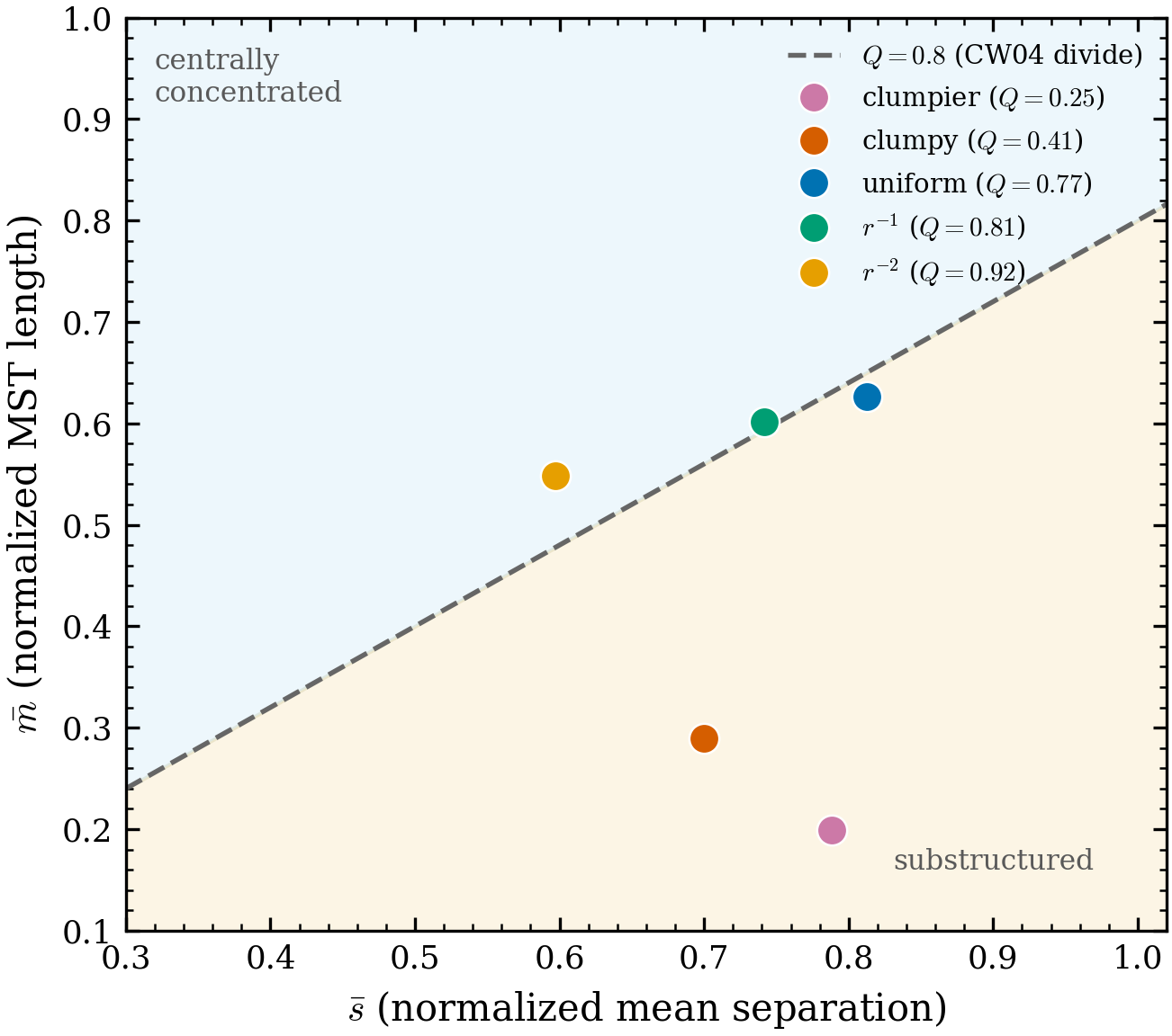
Figure 1:The CW04 plane. The line divides centrally concentrated (, ; above) from substructured (clumpy, clumpier; below) configurations, with the uniform sphere on the divide (). This is the diagnostic’s defining diagram.
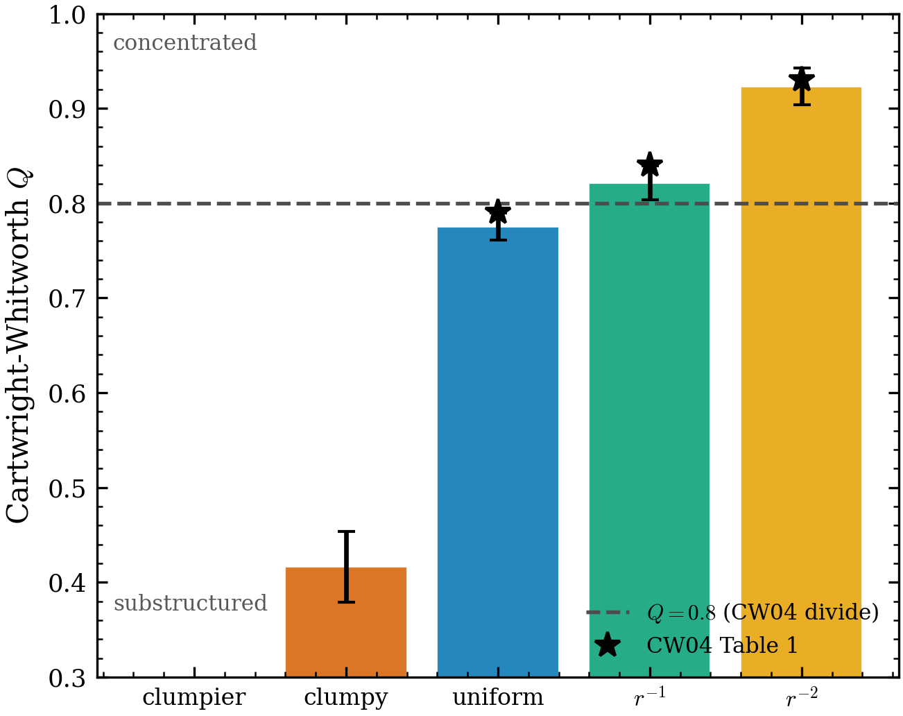
Figure 2:Q ladder vs CW04 Table 1. The exact estimator reproduces CW04 ‘3D0/3D1/3D2’ (stars: ; measured ) and places clumpy/clumpier well below the divide.
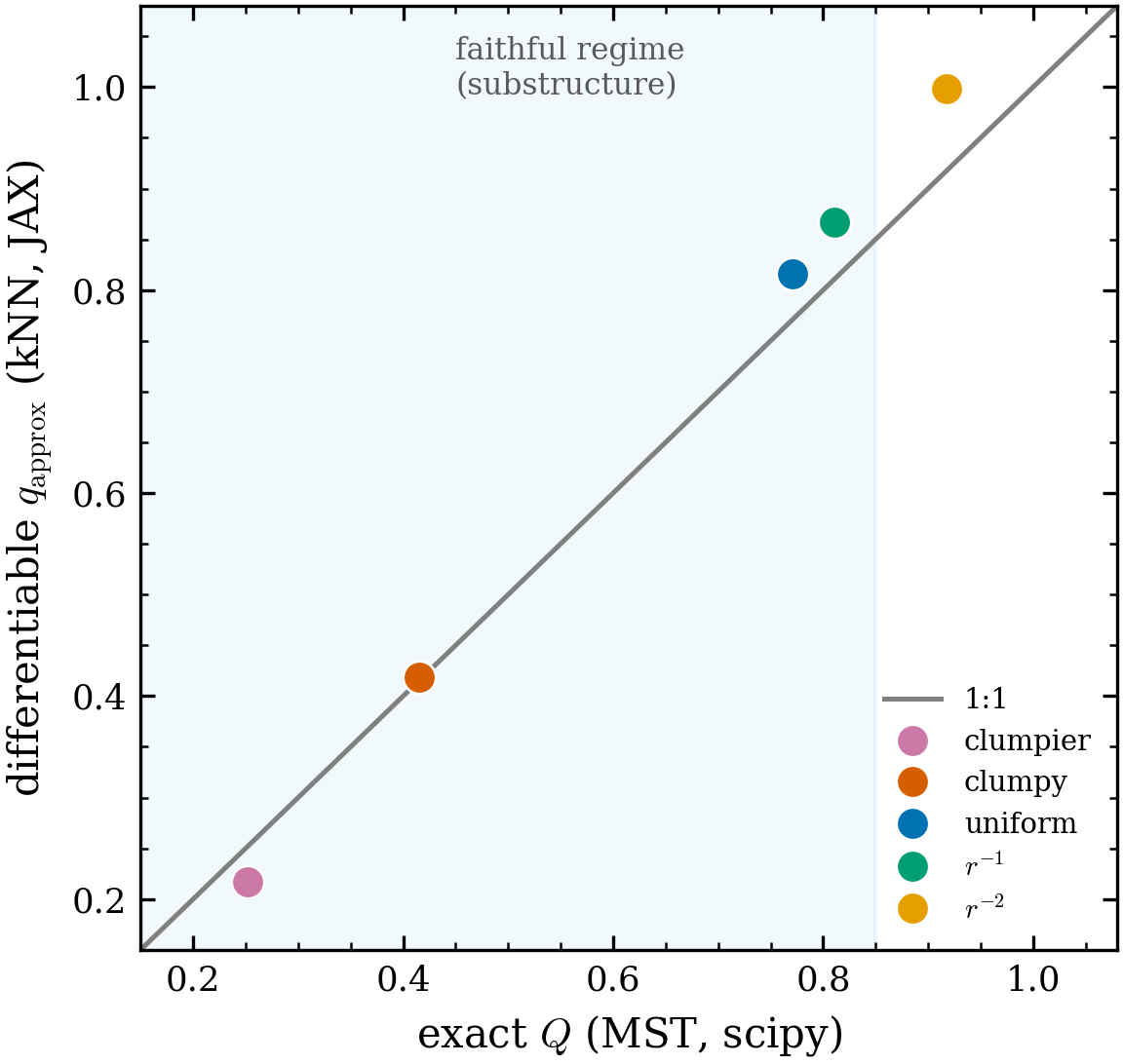
Figure 3:Differentiable vs exact . In the substructure regime (, shaded) — where is used for inference — the JAX kNN estimator tracks the exact scipy MST on the 1:1 line (clumpy +0.004, uniform +0.045). For concentrated profiles () it over-reads by (shown honestly); ordering is preserved throughout.
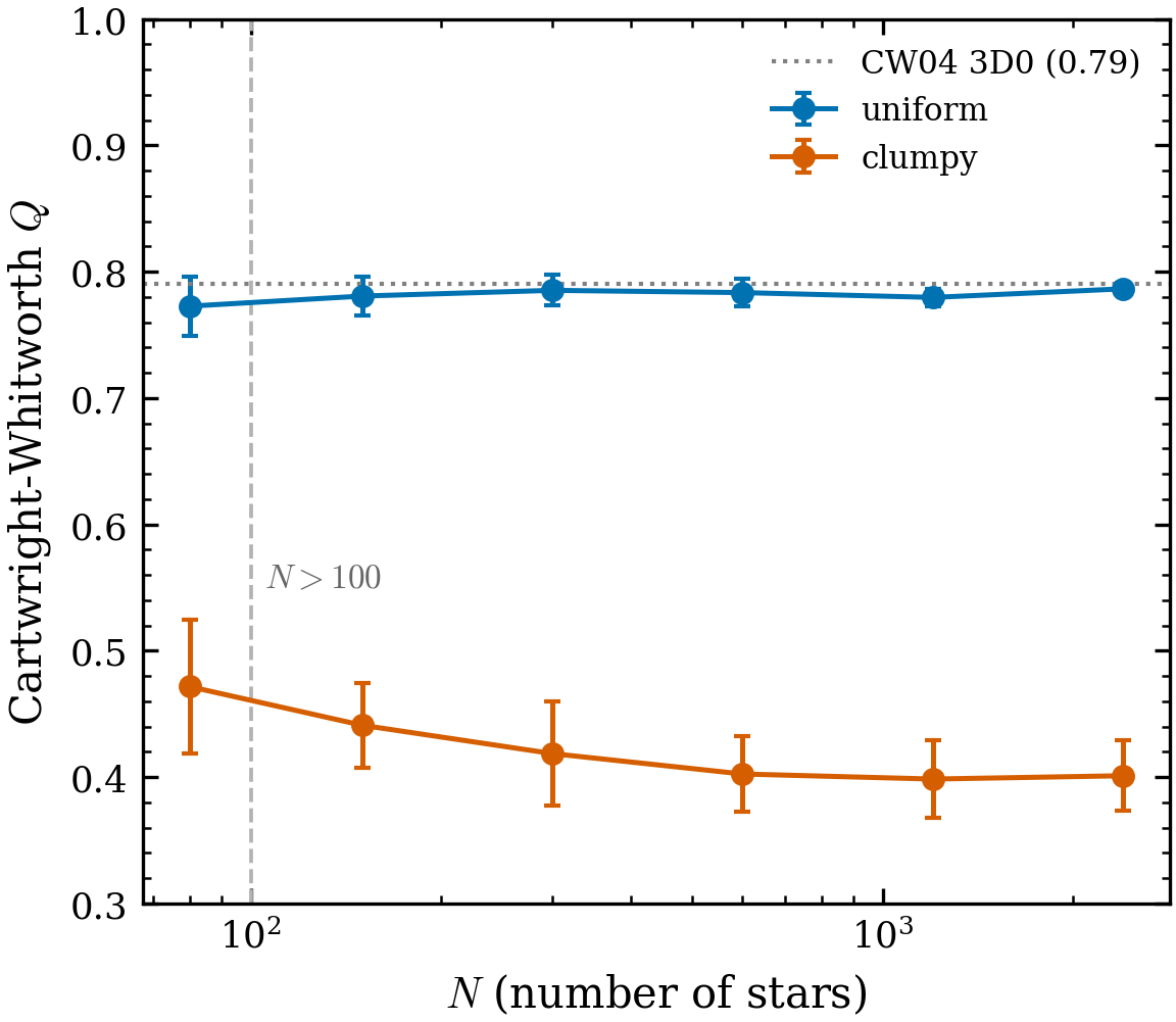
Figure 4:-independence. is approximately independent of for (CW04): the uniform sphere varies by , the clumpy distribution by across –2400.
Differentiability¶
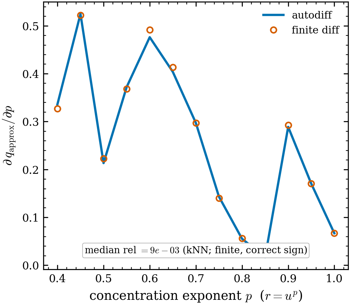
Figure 5: gradient. for a radial
concentration parameter (): autodiff and finite difference agree to a
median . As a kNN estimator, the gradient is exact within a neighbour-set
cell and the finite difference picks up cell-boundary truncation (worst-case
at a boundary); the autodiff gradient is finite and correct-signed
everywhere — usable for gradient-based substructure inference (the reason
q_approx exists alongside the non-differentiable exact compute_q_parameter).
Azimuthal-variation diagnostic (Küpper+2011)¶
compute_azimuthal_variation returns , the
relative scatter of star counts in azimuthal sectors — a cheap substructure
proxy. Test file: tests/validation/test_azimuthal_variation_physics.py (see the
test dashboard for the live per-suite count); figures:
scripts/validate_azimuthal_variation.py.
Property | Tolerance (as tested) | Measured | Anchor |
|---|---|---|---|
Smooth axisymmetric → Poisson floor | 0.059 (floor 0.069) | Poisson counts | |
Monotonic rise with clump fraction | monotone | more clumps ⇒ larger | |
Spans the Küpper range | smooth , clumpy | 0.06 / 0.9 | |
Anti-correlates with CW04 | both detect substructure |
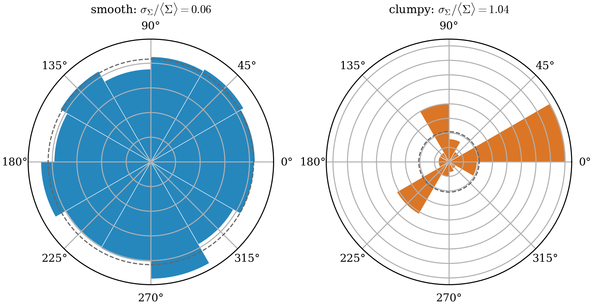
Figure 6:Sector-count histograms. A smooth axisymmetric cluster (left) has nearly flat azimuthal counts (, the Poisson floor); azimuthal clumps (right) give spiky sectors ().
![Response to clumpiness. \sigma_\Sigma/\langle\Sigma\rangle rises monotonically
from the Poisson floor through the range ([0.07,0.76], shaded)
as the azimuthal clump fraction increases. The fractal generator was removed, so the
specific \sigma_\Sigma\!-\!D slope is not reproduced here — only the floor, span, and
monotonic behaviour.](/progenax/build/azimuthal_vs_clumpin-923232c362331f77ba4e5def4af311e1.png)
Figure 7:Response to clumpiness. rises monotonically from the Poisson floor through the Küpper et al. (2011) range (, shaded) as the azimuthal clump fraction increases. The fractal generator was removed, so the specific slope is not reproduced here — only the floor, span, and monotonic behaviour.
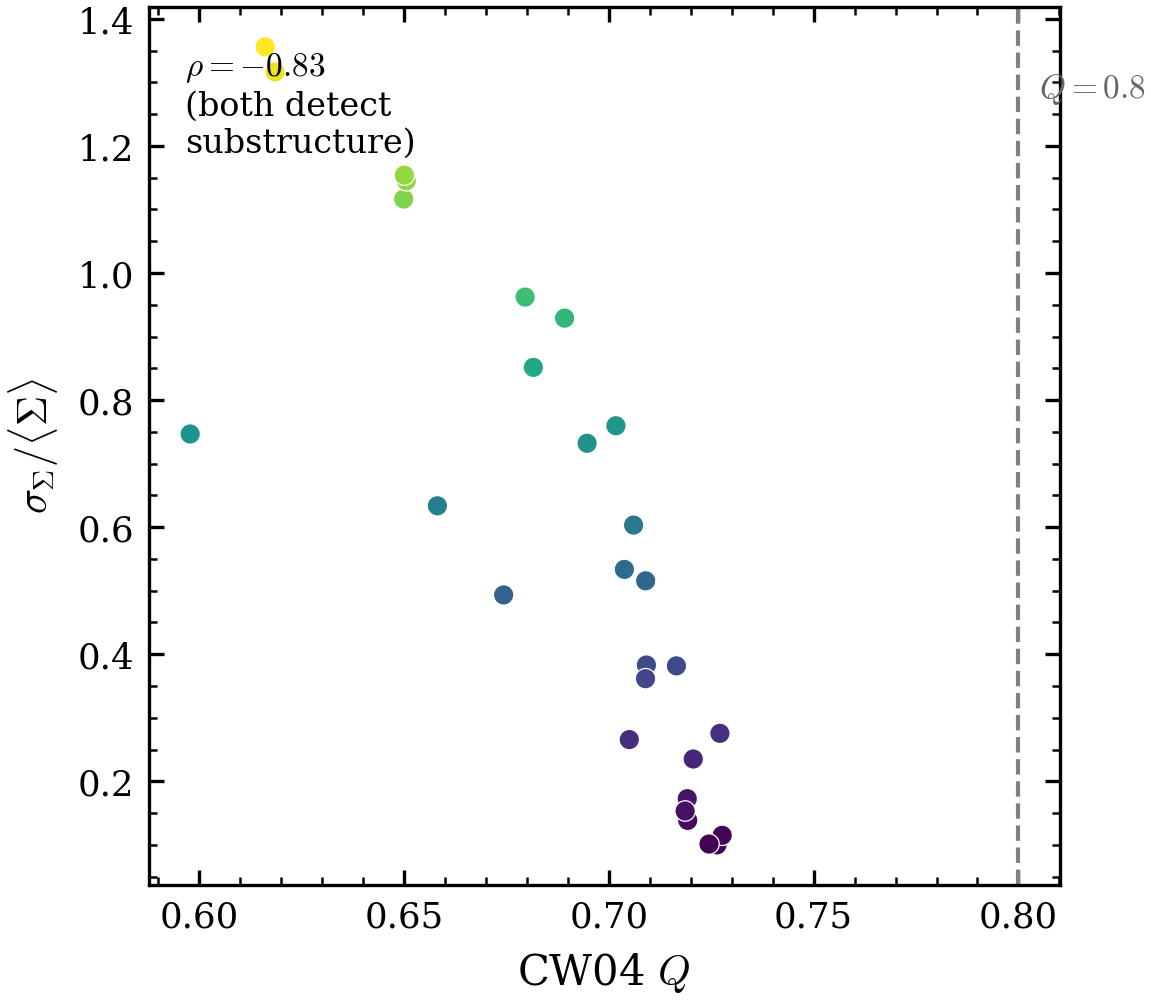
Figure 8:Cross-check vs CW04 . Across a smooth→clumpy sequence the two independent substructure diagnostics anti-correlate (): higher tracks lower .
How to run¶
pytest tests/validation/test_substructure_q_physics.py -q          # ~5 s
pytest tests/validation/test_azimuthal_variation_physics.py -q     # ~1 s
python scripts/validate_substructure_q.py                          # 5 Q figures
python scripts/validate_azimuthal_variation.py                     # 3 azimuthal figures
What this suite does not test¶
Fractal IC generation — removed in the 2026-06 rewrite (no released successor); the turbulent-density method is experimental
gravoturb(src/experimental/, AC6/AC7 — see itsVALIDATION_SUMMARY.md).The Küpper slope — requires fractal-dimension models (generator removed); only the metric’s floor/span/monotonicity is validated.
References¶
The Q diagnostic is Cartwright & Whitworth (2004); the GW04 fractal baseline is Goodwin & Whitworth (2004); the dynamical context is Allison et al. (2009). Theory at Fractal substructure and JAX-native CW04 substructure Q parameter.
- Cartwright, A., & Whitworth, A. P. (2004). The statistical analysis of star clusters. Monthly Notices of the Royal Astronomical Society, 348, 589–598. 10.1111/j.1365-2966.2004.07360.x
- Küpper, A. H. W., Maschberger, T., Kroupa, P., & Baumgardt, H. (2011). Mass segregation and fractal substructure in young massive clusters. Monthly Notices of the Royal Astronomical Society, 417, 2300–2317. 10.1111/j.1365-2966.2011.19412.x
- Goodwin, S. P., & Whitworth, A. P. (2004). The dynamical evolution of fractal star clusters: The survival of substructure. Astronomy and Astrophysics, 413, 929–937. 10.1051/0004-6361:20031529
- Allison, R. J., Goodwin, S. P., Parker, R. J., Portegies Zwart, S. F., de Grijs, R., & Kouwenhoven, M. B. N. (2009). Using the minimum spanning tree to trace mass segregation. Monthly Notices of the Royal Astronomical Society, 395, 1449–1454. 10.1111/j.1365-2966.2009.14508.x