Plummer equilibrium - progenax — differentiable initial conditions for N-body simulations

Plummer equilibrium validation¶

The Plummer suite is the most-tested module in progenax, anchoring the closed-form expressions from Plummer profile. Test file: tests/validation/test_plummer_physics.py (20 tests); JIT/gradient coverage in tests/integration/test_jax_compatibility.py (8 Plummer tests); figures: scripts/validate_plummer.py.

What is verified¶

Each row maps to assertions in test_plummer_physics.py. The Tolerance is the exact bound the test enforces (tests/validation/conftest.py); the Measured value is regenerated by scripts/validate_plummer.py (which prints an expected-vs-measured PASS/FAIL table for every figure).

Property	Tolerance (as tested)	Measured	Anchor
Scale radius $a = r_h\sqrt{2^{2/3}-1}$	10^-6 rel	0.7664 ( $=$ exact)	$M(<r_h)=M/2$
Half-mass fraction (frac $r<r_h$ )	0.03 abs	0.500	definition of $r_h$
$M(<a)/M = 1/2^{3/2}$	0.03 abs	0.3513 (exp 0.3536)	Plummer CDF at $r=a$
Cumulative-mass shape $M(<r)=M\,r^3/(r^2+a^2)^{3/2}$	0.03 abs per radius	max $\|\Delta\mathrm{CDF}\| = 3.6\times10^{-3}$	closed-form CDF
Velocity dispersion $\sigma_{1d}(r)=\sqrt{GM/(6\sqrt{r^2+a^2})}$	$10\%$ rel per bin	max rel $= 1.2\%$	isotropic Jeans / DF 2nd moment
Velocity isotropy $\langle v_x^2\rangle\!\approx\!\langle v_y^2\rangle\!\approx\!\langle v_z^2\rangle$	$5\%$ rel spread	$0.6\%$	isotropic DF
Virial ratio $Q=T/\|V\|$	0.05 abs at $N=5000$	0.5026	$2T+V=0$ , $V=-3\pi GM^2/32a$
Bound fraction ( $v\le v_{\rm esc}$ )	100%	100.00%	$v_{\rm esc}^2=2GM/\sqrt{r^2+a^2}$
Speed law $\langle q^2\rangle$ , $q=v/v_{\rm esc}$	0.02 abs	0.2496 (exp 0.25)	$q^2\sim\mathrm{Beta}(3/2,9/2)$
Speed-law variance $\mathrm{Var}(q^2)$	$15\%$ rel	0.0267 (exp 0.0268)	$\mathrm{Beta}(3/2,9/2)$
Position isotropy $\cos\theta\sim U(-1,1)$ , $\phi\sim U(0,2\pi)$	reduced $\chi^2_\nu\approx1$	$\chi^2_\nu = 0.81,\ 0.75$	spherical symmetry
Sampling differentiability ( $r_h$ , $M$ )	AD $=$ central-FD	rel err $6\times10^{-11}$ , $1.6\times10^{-6}$	`jax.lax.scan` sampling, no `while_loop`

JIT compilation and gradient flow through both position and velocity sampling are additionally verified in tests/integration/test_jax_compatibility.py (8 Plummer tests; test_plummer_jit, test_plummer_grad, test_plummer_df_jit, test_plummer_df_grad, test_plummer_ic_grad_wrt_r_h, …).

Figures¶

Generated by scripts/validate_plummer.py (prints expected-vs-measured PASS/FAIL for every panel; PNG for the web + PDF vector for the paper).

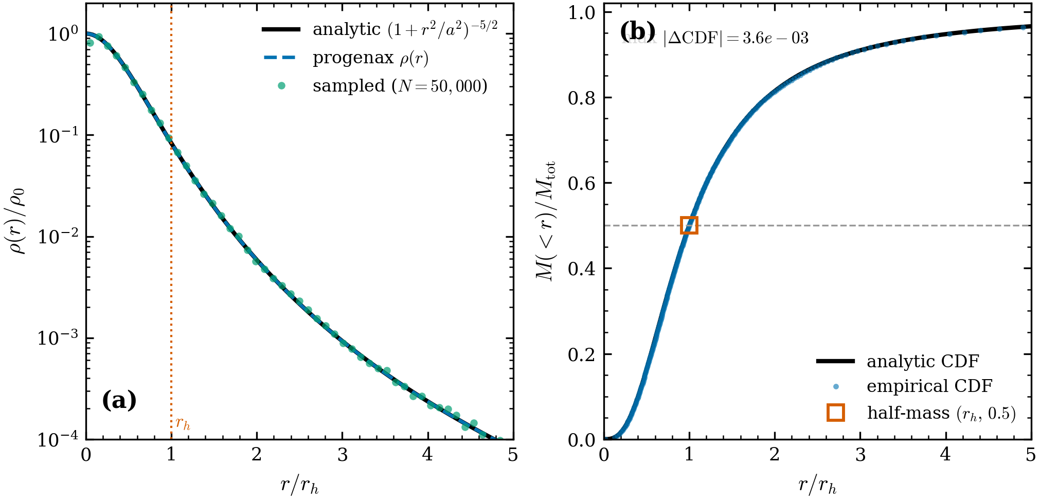
$Density profile and cumulative mass. (a) PlummerProfile.density (dashed) on the analytic (1+r^2/a^2)^{-5/2} (solid) and the N=5\times10^4 sample (points). (b) The empirical CDF tracks the closed form M(<r)=M\,r^3/(r^2+a^2)^{3/2} to max |\Delta\mathrm{CDF}|=3.6\times10^{-3}; the half-mass point (r_h,\,0.5) is marked. The scale radius is a=r_h\sqrt{2^{2/3}-1}=0.7664\,r_h to machine precision.$

Figure 1:Density profile and cumulative mass. (a) PlummerProfile.density (dashed) on the analytic $(1+r^2/a^2)^{-5/2}$ (solid) and the $N=5\times10^4$ sample (points). (b) The empirical CDF tracks the closed form $M(<r)=M\,r^3/(r^2+a^2)^{3/2}$ to max $|\Delta\mathrm{CDF}|=3.6\times10^{-3}$ ; the half-mass point $(r_h,\,0.5)$ is marked. The scale radius is $a=r_h\sqrt{2^{2/3}-1}=0.7664\,r_h$ to machine precision.

Velocity-space equilibrium. (a) Sampled \sigma_{1d}(r) on the analytic
\sqrt{GM/(6\sqrt{r^2+a^2})} (per-bin rel \le 1.2\%). (b) Every velocity
satisfies v\le v_{\rm esc}(r) — 100% bound. (c) The unscaled IC sits at
virial Q=0.5026 (tested to \pm0.05): the matched DF is a true
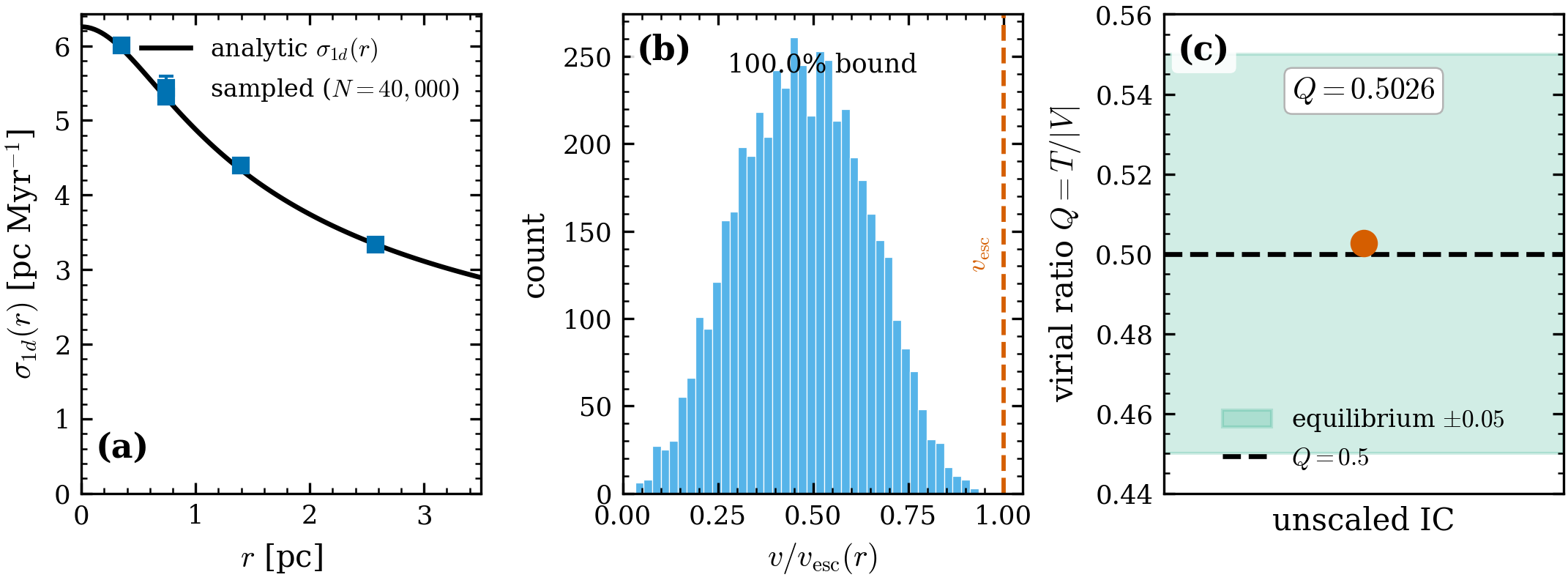
equilibrium with no external rescale. — Figure 2:**Velocity-space equilibrium.** (a) Sampled $\sigma_{1d}(r)$ on the analytic $\sqrt{GM/(6\sqrt{r^2+a^2})}$ (per-bin rel $\le 1.2\%$ ). (b) Every velocity satisfies $v\le v_{\rm esc}(r)$ — **100% bound**. (c) The unscaled IC sits at virial **$Q=0.5026$** (tested to $\pm0.05$ ): the matched DF is a true equilibrium with **no external rescale**.

The Plummer speed law. The sampled q^2=(v/v_{\rm esc})^2 histogram
(N=4\times10^4) overlays the exact \mathrm{Beta}(3/2,9/2) density — the
distribution rejection-sampling reproduces. Measured
\langle q^2\rangle = 0.2496 (exact 0.25) and \mathrm{Var}(q^2)=0.0267
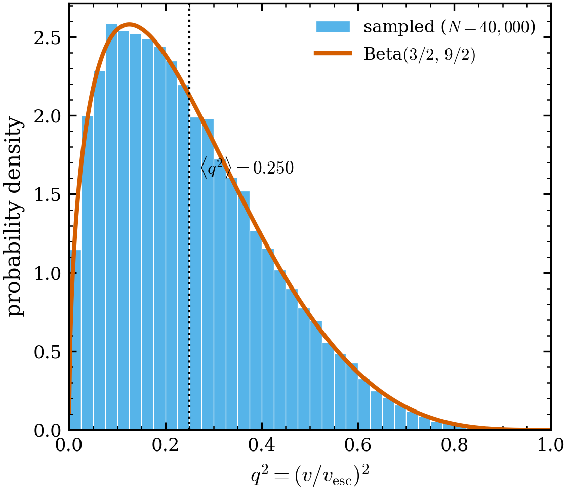
(exact 0.0268). — Figure 3:**The Plummer speed law.** The sampled $q^2=(v/v_{\rm esc})^2$ histogram ( $N=4\times10^4$ ) overlays the exact $\mathrm{Beta}(3/2,9/2)$ density — the distribution Aarseth *et al.* (1974) rejection-sampling reproduces. Measured $\langle q^2\rangle = 0.2496$ (exact 0.25) and $\mathrm{Var}(q^2)=0.0267$ (exact 0.0268).

Position isotropy. (a) \cos\theta and (b) \phi of the sampled positions
are flat against their uniform expectations U(-1,1) and U(0,2\pi), with
reduced \chi^2_\nu = 0.81 and 0.75 (consistent with unity). Velocity
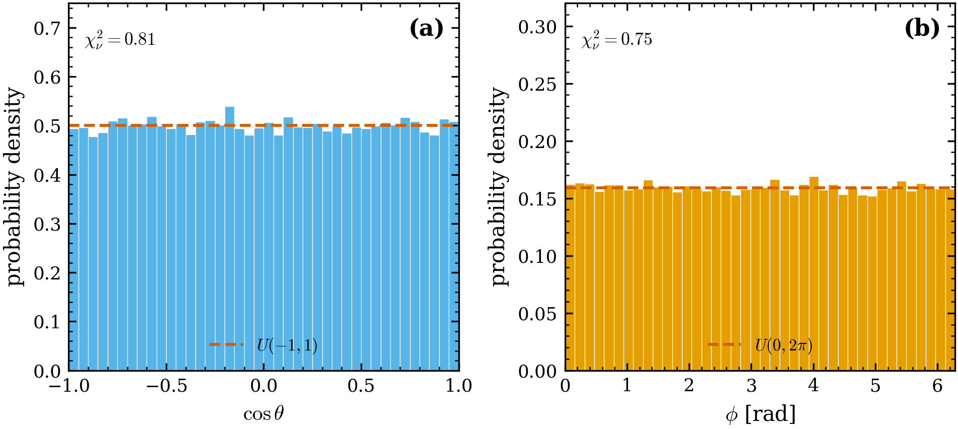
isotropy \langle v_i^2\rangle agrees to 0.6\% (printed by the script). — Figure 4:**Position isotropy.** (a) $\cos\theta$ and (b) $\phi$ of the sampled positions are flat against their uniform expectations $U(-1,1)$ and $U(0,2\pi)$ , with reduced $\chi^2_\nu = 0.81$ and 0.75 (consistent with unity). Velocity isotropy $\langle v_i^2\rangle$ agrees to $0.6\%$ (printed by the script).

Differentiability¶

The Plummer IC pipeline is built for gradient-based inference: the model observables a likelihood uses — the density profile $\rho(r)$ and the velocity scale $\sigma_0\propto\sqrt{GM}$ — are differentiable w.r.t. the structural parameters $(r_h, M)$ that one fits to data.

Gradient validation (autodiff vs central finite difference). (a)
\partial\log\rho(1\,\mathrm{pc})/\partial r_h and (b)
\partial\sigma_0/\partial M_{\rm tot}: autodiff (line) and finite difference
(circles) agree to max rel err 6\times10^{-11} and 1.6\times10^{-6}, so
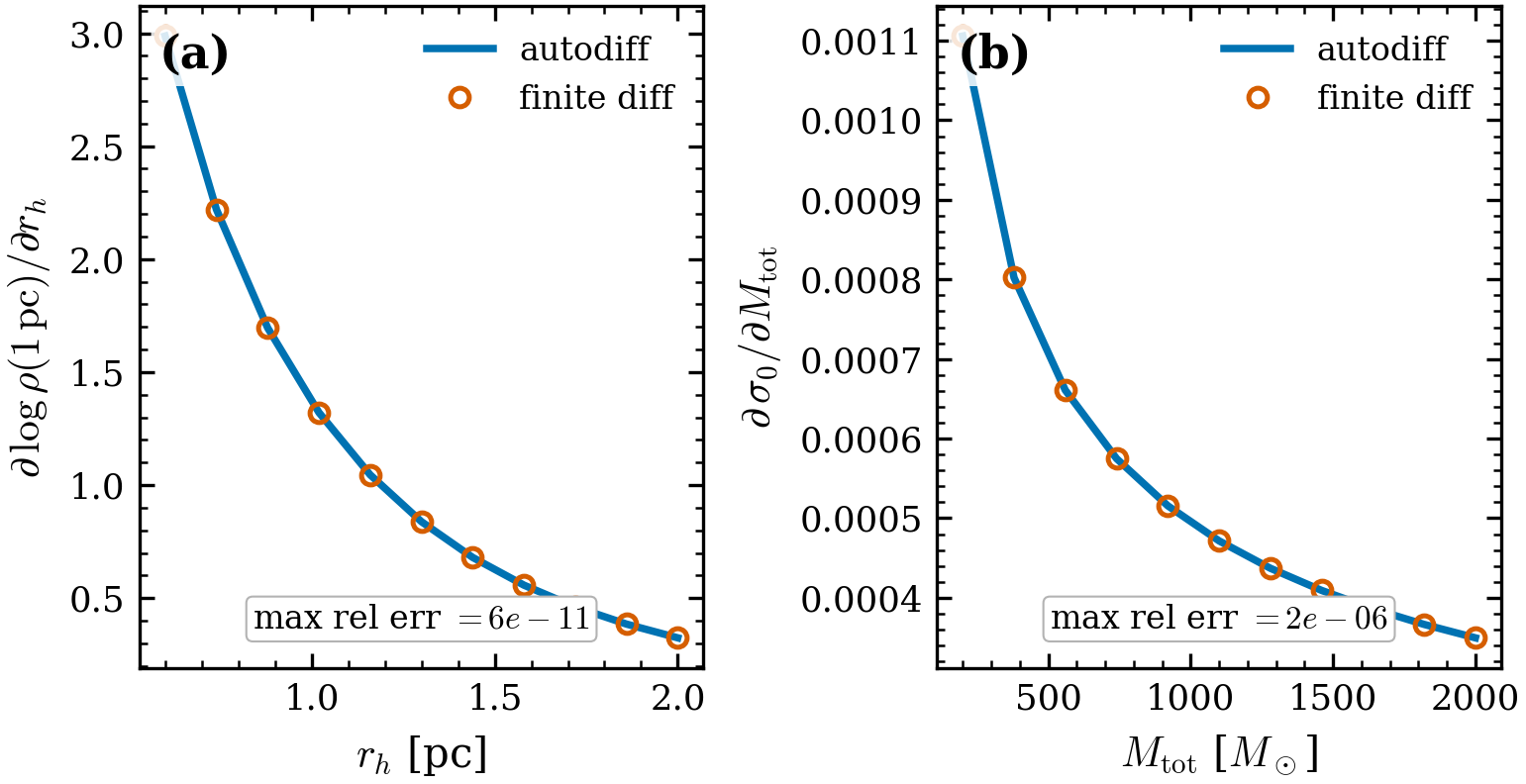
(r_h, M_{\rm tot}) can be inferred jointly by gradient descent or HMC. — Figure 5:**Gradient validation (autodiff vs central finite difference).** (a) $\partial\log\rho(1\,\mathrm{pc})/\partial r_h$ and (b) $\partial\sigma_0/\partial M_{\rm tot}$ : autodiff (line) and finite difference (circles) agree to **max rel err $6\times10^{-11}$** and $1.6\times10^{-6}$ , so $(r_h, M_{\rm tot})$ can be inferred jointly by gradient descent or HMC.

How to run¶

# physics tests (20 tests, ~4 s on CPU)
pytest tests/validation/test_plummer_physics.py -q

# regenerate the five figures with PASS/FAIL tables
python scripts/validate_plummer.py

What this suite does not test¶

Long-term evolution — covered by gravax integration tests, not here. progenax validates ICs at $t=0$ .
Multi-mass equipartition — single-mass Plummer is covered; the multi-mass / anisotropic generalization (the differentiable lowered-model family) is planned progenax work following Gieles & Zocchi (2015) — see the roadmap. It is not delegated to an external package.
Tidal truncation — covered separately in Tidal truncation validation.

References¶

The Plummer derivations come from Plummer (1911); the inverse-CDF radius draw and the $\mathrm{Beta}(3/2,9/2)$ speed law follow Aarseth et al. (1974). The full theoretical content is at Plummer profile.

References¶

Aarseth, S. J., Henon, M., & Wielen, R. (1974). A comparison of numerical methods for the study of star cluster dynamics. Astronomy and Astrophysics, 37, 183–187.
Gieles, M., & Zocchi, A. (2015). A family of lowered isothermal models. Monthly Notices of the Royal Astronomical Society, 454, 576–592. 10.1093/mnras/stv1848
Plummer, H. C. (1911). On the problem of distribution in globular star clusters. Monthly Notices of the Royal Astronomical Society, 71, 460–470. 10.1093/mnras/71.5.460