ZAMS relations validation - progenax — differentiable initial conditions for N-body simulations

progenax.stellar provides the Tout et al. (1996) zero-age main-sequence (ZAMS) relations — mass to luminosity, radius, effective temperature, and surface gravity, plus a differentiable inverse $L \to M$ — as five pure, array-aware, autodiff-ready functions. They are the metallicity-dependent photometric placeholder for the eventual startrax stellar tracks: the bridge from a sampled IMF to a colour-magnitude diagram or a mass–luminosity inference. Test files: tests/validation/test_zams_physics.py (34 tests, validation tier) and tests/unit/stellar/test_zams.py (unit tier); figures: scripts/validate_zams.py.

The relations¶

The luminosity and radius are rational functions of mass with metallicity-dependent coefficients (each coefficient, except the scalar $\nu$ , is a degree-4 polynomial in $\zeta = \log_{10}(Z/Z_\odot)$ , $Z_\odot = 0.02$ ):

\frac{L}{L_\odot} = \frac{\alpha M^{5.5} + \beta M^{11}} {\gamma + M^{3} + \delta M^{5} + \epsilon M^{7} + \zeta M^{8} + \eta M^{9.5}}

(1)

\frac{R}{R_\odot} = \frac{\theta M^{2.5} + \iota M^{6.5} + \kappa M^{11} + \lambda M^{19} + \mu M^{19.5}} {\nu + \xi M^{2} + o\,M^{8.5} + M^{18.5} + \pi M^{19.5}}

(2)

with $M \equiv M/M_\odot$ . The effective temperature and surface gravity are not independent fits — they follow from $L$ and $R$ by physics:

T_{\rm eff} = \left(\frac{L}{4\pi R^2 \sigma}\right)^{1/4}, \qquad \log g = \log_{10}\!\left(\frac{G M}{R^2}\right) \ \text{(cgs)}.

(3)

The inverse $L \to M$ is a fixed-iteration Newton solve in a jax.lax.scan (not a while_loop), so it is differentiable: the analytic slope $dL/dM$ is obtained by jax.grad of the forward relation, and the round-trip $M \to L \to M$ recovers the mass to machine precision over the whole fitted range.

What is verified¶

Rows map to tests/validation/test_zams_physics.py; Measured values are regenerated by scripts/validate_zams.py (which prints expected-vs-measured PASS/FAIL per figure and exits non-zero on any failure). Each check uses an independent oracle — the PDF-verified algebra, the Stefan-Boltzmann/Newton closure, monotonicity, or the forward relation the inverse must undo — not the formula’s own restatement.

Property	Tolerance (as tested)	Measured	Anchor
Solar $L(1\,M_\odot, 0.02)$	within $3\%$ (paper’s solar $L$ accuracy)	$0.6977\,L_\odot$	PDF-verified Table 1 algebra
Solar $R(1\,M_\odot, 0.02)$	within $1.2\%$ (paper’s solar $R$ accuracy)	$0.8882\,R_\odot$	PDF-verified Table 2 algebra
Solar $T_{\rm eff}(1\,M_\odot)$	$=$ computed value to 10^-6	$5597\,{\rm K}$	Stefan-Boltzmann of $L,R$
Solar $\log g(1\,M_\odot)$	$=$ computed value to 10^-6	$4.541\,{\rm dex}$	$g = GM/R^2$ (cgs)
$T_{\rm eff}$ vs hand Stefan-Boltzmann	max rel $< 10^{-10}$	0 (machine-exact)	$4\pi R^2 \sigma T_{\rm eff}^4 = L$
$L(M)$ strictly monotone over $[0.1,100]\,M_\odot$	all $\Delta L > 0$	True	homology (invertibility)
Inverse round-trip $M \to L \to M$	rel $< 10^{-5}$	$5\times10^{-16}$	forward $L(M)$
Inverse $dM/dL$ (AD vs FD)	rel $< 10^{-4}$	$1.6\times10^{-11}$	central finite difference
Metal-poor is bluer/brighter at fixed $M$	$L_{Z=10^{-3}} > L_{Z=0.02}$	$1.46 > 0.70\,L_\odot$	lower opacity (homology)

Validity & accuracy envelope¶

The Tout et al. (1996) fits are valid for $0.1 \le M/M_\odot \le 100$ and $10^{-4} \le Z \le 0.03$ . Over that box the luminosity is accurate to $< 7.5\%$ ( $< 3\%$ at solar $Z$ ) and the radius to $< 5\%$ ( $< 1.2\%$ at solar); the worst cases are $L \sim 14\%$ at $M=0.1\,M_\odot,\,Z=0.0003$ and $R \sim 5\%$ at $M=0.52\,M_\odot,\,Z=0.001$ . Metallicity extrapolation is forbidden — the rational functions go negative outside the fitted $Z$ range — so stellar.py clips $Z$ to $[10^{-4}, 0.03]$ as the paper’s explicit guidance, not an arbitrary guard.

Figures¶

Generated by scripts/validate_zams.py (PASS/FAIL per panel; PNG raster for this site, PDF vector for papers).

ZAMS luminosity L(M) over the full fitted range at three metallicities (solar
Z=0.02, Z=0.001, Z=10^{-4}). The solar anchor L(1\,M_\odot,0.02)=0.698\,L_\odot
(star) reproduces the PDF-verified value, and L(M) is strictly monotone — the homology
property that makes the luminosity invertible. Metal-poor tracks sit above the solar
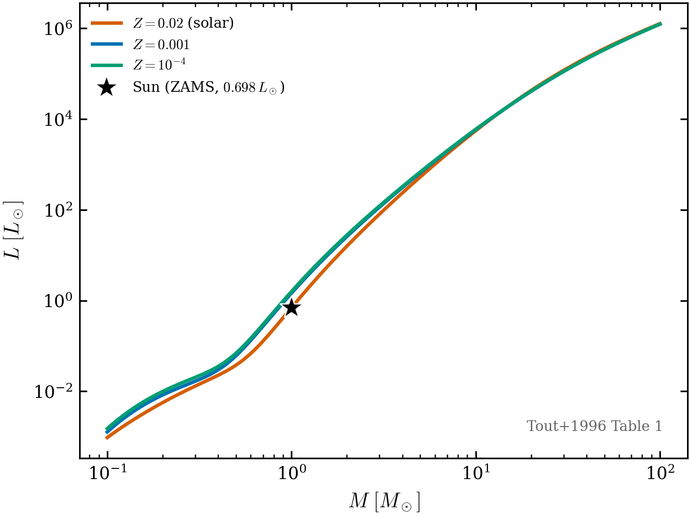
one (lower opacity ⇒ brighter at fixed mass). — Figure 1:ZAMS luminosity $L(M)$ over the full fitted range at three metallicities (solar $Z=0.02$ , $Z=0.001$ , $Z=10^{-4}$ ). The solar anchor $L(1\,M_\odot,0.02)=0.698\,L_\odot$ (star) reproduces the PDF-verified value, and $L(M)$ is strictly monotone — the homology property that makes the luminosity invertible. Metal-poor tracks sit **above** the solar one (lower opacity ⇒ brighter at fixed mass).

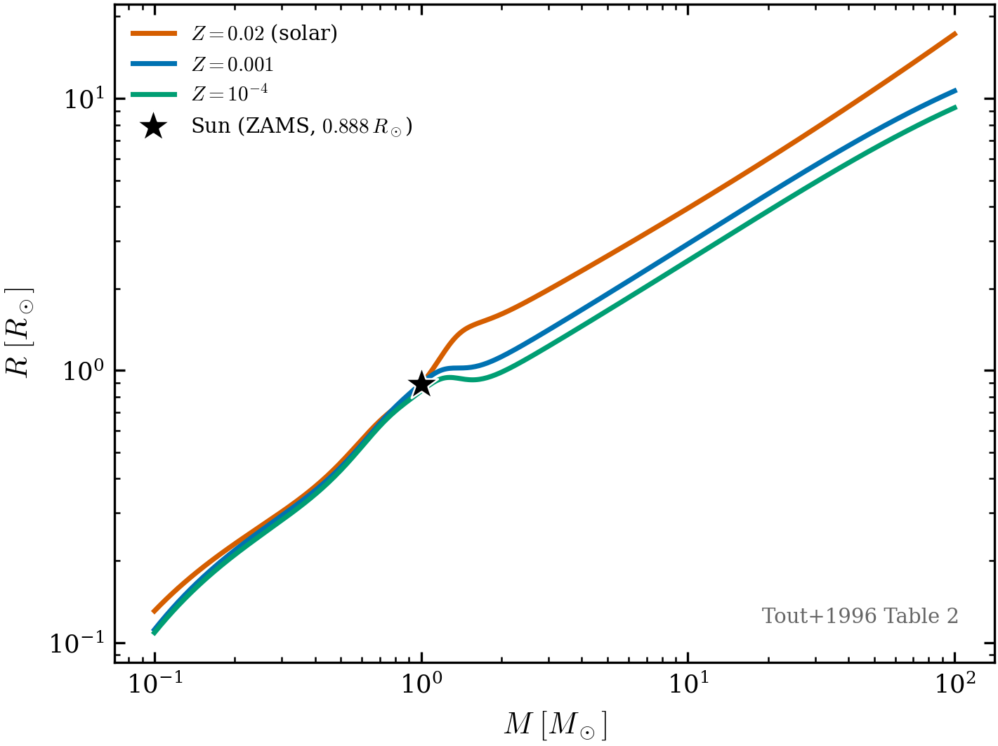
ZAMS radius R(M) over the fitted range at the same three metallicities. The solar
anchor R(1\,M_\odot,0.02)=0.888\,R_\odot (star) matches the PDF-verified value; R(M)
stays finite and positive across the whole range. — Figure 2:ZAMS radius $R(M)$ over the fitted range at the same three metallicities. The solar anchor $R(1\,M_\odot,0.02)=0.888\,R_\odot$ (star) matches the PDF-verified value; $R(M)$ stays finite and positive across the whole range.

ZAMS effective temperature T_{\rm eff}(M) from Stefan-Boltzmann. The module curve
(points) lies exactly on the hand-computed closure T_{\rm eff}=(L/4\pi R^2\sigma)^{1/4}
(line) to machine precision — an independent check that the physics, not just the
coefficients, is wired correctly. The ZAMS Sun sits at 5597\,{\rm K} (cooler and smaller
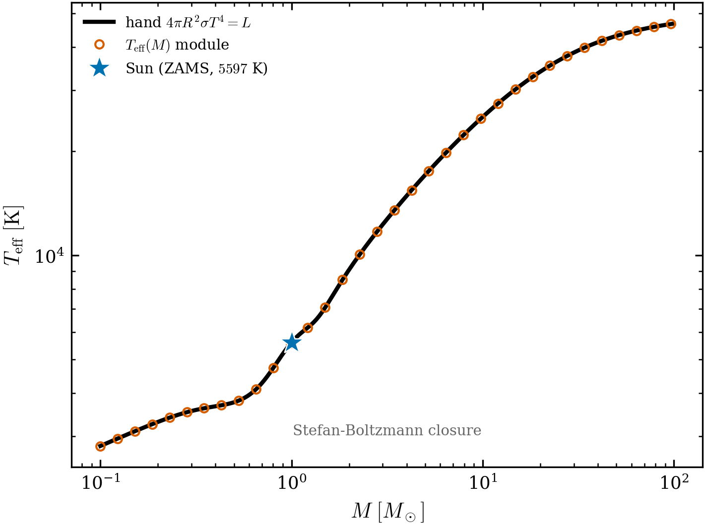
than today’s 5772\,{\rm K} Sun). — Figure 3:ZAMS effective temperature $T_{\rm eff}(M)$ from Stefan-Boltzmann. The module curve (points) lies exactly on the hand-computed closure $T_{\rm eff}=(L/4\pi R^2\sigma)^{1/4}$ (line) to machine precision — an independent check that the *physics*, not just the coefficients, is wired correctly. The ZAMS Sun sits at $5597\,{\rm K}$ (cooler and smaller than today’s $5772\,{\rm K}$ Sun).

The ZAMS in the Hertzsprung-Russell plane (\log L vs \log T_{\rm eff}, hot/blue to the
left) at three metallicities — the Fig. 5 view. The solar track is
marked with mass ticks (0.3–30\,M_\odot) and the ZAMS Sun. Lower-metallicity ZAMS
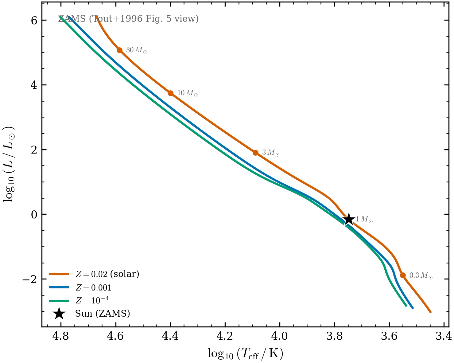
loci are hotter at fixed mass (bluer), as expected from the reduced opacity. — Figure 4:The ZAMS in the Hertzsprung-Russell plane ( $\log L$ vs $\log T_{\rm eff}$ , hot/blue to the left) at three metallicities — the Tout *et al.* (1996) Fig. 5 view. The solar track is marked with mass ticks (0.3– $30\,M_\odot$ ) and the ZAMS Sun. Lower-metallicity ZAMS loci are hotter at fixed mass (bluer), as expected from the reduced opacity.

Left: the inverse solve M_{\rm rec}=L^{-1}(L(M)) lies on y=x across
[0.1,100]\,M_\odot. Right: the round-trip relative residual stays at the
floating-point floor (\sim 5\times10^{-16}, well under the 10^{-5} tolerance) — the
fixed-iteration Newton/scan invert reaches machine precision, and its gradient dM/dL
agrees with a central finite difference to 1.6\times10^{-11} (the inference-grade
differentiability the inverse exists for). — Figure 5:**Left:** the inverse solve $M_{\rm rec}=L^{-1}(L(M))$ lies on $y=x$ across $[0.1,100]\,M_\odot$ . **Right:** the round-trip relative residual stays at the floating-point floor ( $\sim 5\times10^{-16}$ , well under the 10^-5 tolerance) — the fixed-iteration Newton/scan invert reaches machine precision, and its gradient $dM/dL$ agrees with a central finite difference to $1.6\times10^{-11}$ (the inference-grade differentiability the inverse exists for).

Differentiability¶

All five relations flow finite gradients (the Fisher-information requirement for mass-function and CMD inference). The forward $\partial L/\partial M$ , $\partial R/\partial M$ , $\partial T_{\rm eff}/\partial M$ , $\partial \log g/\partial M$ and the inverse $\partial M/\partial L$ (through the lax.scan Newton) are each registered in the release gradient gate as measured AD-vs-FD cases; the inverse case audits the gradient through the fixed-iteration solver, confirming the scan (not a while_loop) keeps the invert differentiable.

References¶

Tout, C. A., Pols, O. R., Eggleton, P. P., & Han, Z. (1996). Zero-age main-sequence radii and luminosities as analytic functions of mass and metallicity. Monthly Notices of the Royal Astronomical Society, 281, 257. 10.1093/mnras/281.1.257