The idea
The classical truncated-isothermal models — Woolley (no energy truncation), King (1966) (a linear lowered Maxwellian), and Wilson (a quadratic lowered form) — are members of one family distinguished by how sharply the distribution function is truncated near the escape energy. Gieles & Zocchi (2015) made this explicit with a single continuous truncation parameter : their LIMEPY DF reads
with recovering the Woolley cutoff, the King model, and the Wilson model, interpolating smoothly in between. The same framework extends naturally to multiple mass components (each mass group its own , sharing one potential) and to radial anisotropy (an Osipkov–Merritt / Michie term).
The coupled multi-component equilibrium
progenax generalizes the single-mass solve to components sharing one dimensionless potential , . The model-defining insight is that a component’s single free Engine-A scale is its velocity-scale ratio
so component sees the shared potential at the rescaled depth and contributes a density (the “lowered exponential” of Gieles & Zocchi (2015), Appendix B), giving the coupled Poisson equation
with the central density fractions (). A colder component () feels a deeper effective well and concentrates — as a genuine equilibrium, not a post-hoc radial reshuffling. Mass segregation is then the equipartition convenience
(Gieles & Zocchi (2015), Eqs. 24–26): is the standard partial-equipartition choice, collapses every component to the single-mass model exactly (the cleanest oracle). The representative stellar masses are otherwise decoupled labels — the structure depends only on , so equal-mass populations of different concentration (GC 1G/2G, halo+core, binaries-vs-singles) set directly.
Per-component radial anisotropy enters as an Osipkov–Merritt / Michie term
with its own anisotropy radius
(Michie (1963); Merritt (1985)); the anisotropic density is
evaluated by an exact, numerically stable 1-D quadrature (the bounded
Poisson sum) because JAX’s hyp1f1 is NaN for arguments
.
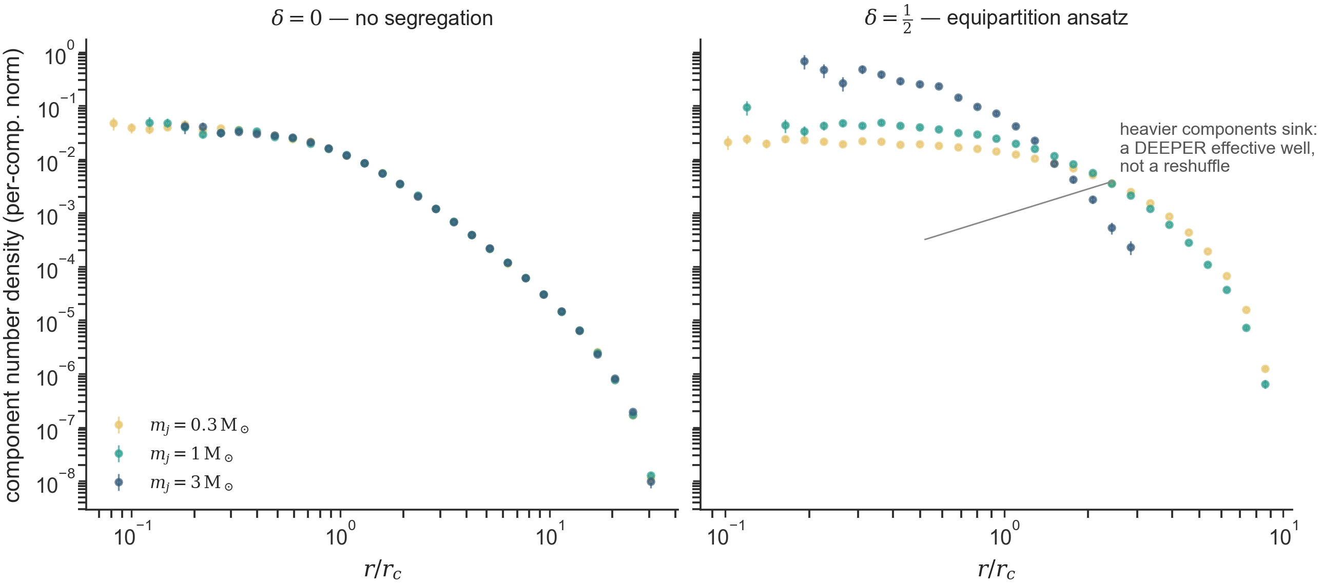
Figure 1:Mass segregation as a genuine equilibrium (seed 31, stars,
). At every component’s
density collapses onto the same profile — the single-mass oracle, visually
exact. At the heavy component concentrates (and the
whole model restructures: note the smaller ) while the light component
extends: heavier components feel a DEEPER effective well
— segregation is in the DF, not a positional reshuffle.
Regenerate: python -m laboratory.icviz --only engine-a-segregation.
Entry points
The family is exposed through three MultiComponentCluster constructors
(see Multi-component populations for the engine map and
Two-component populations — worked examples for a worked example):
from progenax import MultiComponentCluster

# General: per-component velocity-scale ratios (GC 1G/2G, halo+core, ...)
model = MultiComponentCluster.from_components(
    alpha_j=[0.5, 0.5], w_j=[0.7, 1.0], m_j=[1.0, 1.0], W0=7.0, g=1.0)

# Mass segregation as equipartition: w_j = mu_j^(-delta)
model = MultiComponentCluster.from_mass_segregation(
    alpha_j=[0.6, 0.4], m_j=[0.3, 3.0], W0=7.0, g=1.0, delta=0.5)

# IMF-driven: bin the IMF, eigenvalue-solve for the alpha_j that
# reproduce the per-bin mass budget
model = MultiComponentCluster.from_imf(imf, n_comp=8, W0=7.0, g=1.0, delta=0.5)

ic = model.sample_cluster(key, n_stars=50_000)   # ICResult with component_id
sample_cluster draws every star from its component’s lowered DF at the
rescaled potential and velocity scale — no external
virial rescale anywhere: each component is individually virial
() and the sampled cluster is globally virial for any mass
spectrum. The unequal-mass two-population regression measures theory
, sampled global within and
per-component within at test resolution. The single-mass
corners were validated against the released models directly: isotropic
King, anisotropic
Michie, both with unscaled.
Check yourself
1. Why does shrink when segregation turns on?
Compare the two panels’ radial extents in Figure 1. Turning on makes the heavy component colder (), deepening the central potential it generates — at fixed the whole model becomes more concentrated and its dimensionless truncation moves inward.
2. Verify the degeneracy numerically
Sample from_mass_segregation(..., delta=0.0) and run a two-sample KS test
between the radii of any two components — it should be consistent with one
distribution (the components differ only by their decoupled mass labels).
The DF-table performance layer
The anisotropic density quadrature is the 86% hotspot of the coupled solve,
and per-star speed draws dominated sampling. Phase 1.5 replaced both with
three differentiable table primitives in profiles/limepy_tables.py — with
the exact quadrature retained everywhere as a selectable oracle
(aniso_method="quadrature"), and every approximation budget asserted in
tests:
DF tables — design and measured budgets (every row is a regression test against the retained quadrature oracle).
Table | Grid / scheme | Measured vs oracle |
|---|---|---|
| grid, tensor-product 4-point cubic Lagrange (); 512×96 pointwise, 160×40 in-solve | density (budget 10-5); solve over 3 configs; mass CDF |
| 256×256 on ; row-relative CDF normalization; gated to | speed moments vs DF quadrature |
| 192×48×192 on ; the angular conditional stays exact | speed moments ; sampled the DF’s own quadrature within 0.06 (unchanged) |
Measured speedups (warm, two-component, ): anisotropic
construction 5.6× faster (957 → 170 ms); sampling at :
isotropic 67× (0.48 µs/star), anisotropic 21.7× (2.9 µs/star). The
anisotropic table build dominates at small — break-even is ~3k stars.
Crucially, the equilibrium oracle component_virial_ratios is deliberately
quadrature-only (it must not share the approximation it checks): a
table-built model proves against it.
Why progenax reimplemented it (rather than depend on LIMEPY)
Gieles & Zocchi (2015) is the reference formalism, and the published limepy
code is the standard numpy/scipy implementation. progenax does not wrap or
depend on it, for one decisive reason: limepy is not differentiable. The
entire progenax thesis is JAX-native, end-to-end-differentiable initial
conditions, so that structural parameters can be inferred from data by
gradient descent or HMC (see Differentiability rules).
The implemented family delivers exactly this: a single continuous parameter vector — — can be fit jointly to an observed cluster, with itself a fitted quantity that selects the truncation sharpness the data prefer (King-vs-Wilson as a posterior, not a modelling choice). flows through the coupled Poisson solve and through the DF tables: AD agrees with finite differences to , and the table-backed gradient agrees with the quadrature-backed gradient to . The anisotropic and mass-segregation parameters are likewise differentiable through construction and sampling.
Delivered scope
Capability | Status | Measured |
|---|---|---|
King (), single mass | ✅ released (King) | vs King (1966) Table II, |
Continuous (Woolley King Wilson) | ✅ delivered ( | corner King (iso) / Michie (aniso), unscaled |
Multi-mass / multi-component equilibrium (per-component ) | ✅ delivered ( | theory ; sampled global , per-component |
Radial anisotropy per component (, Osipkov–Merritt / Michie) | ✅ delivered | sampled DF quadrature within 0.06 |
DF-table acceleration (oracle-backed) | ✅ delivered (Phase 1.5) | 5.6× construction; 67× (iso) / 21.7× (aniso) sampling at |
Differentiable structural inference | ✅ delivered | AD-vs-FD ; table-AD quadrature-AD |
Relationship to the other roadmap item
This is independent of, but complementary to, the now-resolved differentiable tidal radius (Differentiable King tidal radius ()): the scalar already carries a finite, exact gradient through the unclamped crossing. In the unified family is a function of ; the same implicit-function-theorem treatment of the crossing carries over to the generalization unchanged.
Implementation, validation & references
In code:
src/progenax/cluster/multicomponent.py(MultiComponentClusterand the coupled-Poisson coresolve_multicomponent_limepy), with the lowered-density kernel insrc/progenax/profiles/limepy_multimass.pyand the DF-table layer insrc/progenax/profiles/limepy_tables.py. See theMultiComponentClusterAPI.Validated in: multimass equilibrium — per-component , the single-mass King/Michie corners, and the AD-vs-FD gradient checks for .
Primary sources: Gieles & Zocchi (2015) (the LIMEPY lowered-model formalism); single-model members are King (1966) (with Woolley 1954 / Wilson 1975 for the endpoints), and anisotropy follows Michie (1963) and Merritt (1985). Full notes in the bibliography: Gieles & Zocchi 2015 and King 1966.
- King, I. R. (1966). The structure of star clusters. III. Some simple dynamical models. The Astronomical Journal, 71, 64–75. 10.1086/109857
- Gieles, M., & Zocchi, A. (2015). A family of lowered isothermal models. Monthly Notices of the Royal Astronomical Society, 454, 576–592. 10.1093/mnras/stv1848
- Michie, R. W. (1963). On the distribution of high energy stars in spherical stellar systems. Monthly Notices of the Royal Astronomical Society, 125, 127–139. 10.1093/mnras/125.2.127
- Merritt, D. (1985). Spherical stellar systems with spheroidal velocity distributions. The Astronomical Journal, 90, 1027–1037. 10.1086/113810