Performance & memory

The 2026-06 memory batch replaced the two kernels that could exhaust RAM on a single workstation: the dense $(N,N,3)$ pairwise virial kernels in progenax.dynamics.virial, and the per-star quadrature speed sampler in the standalone anisotropic velocity DFs. Every number on this page is measured, not estimated — the benchmark checks out the pre-batch commit (0dd1cd9) into a read-only git worktree and runs both code versions live in subprocess-isolated cases on the same machine (Apple Silicon, macOS, float64, eager mode; medians of 5 timed calls after one warm-up). Reproduce with:

env -u VIRTUAL_ENV uv run --no-sync python scripts/benchmark_batch_a.py
env -u VIRTUAL_ENV uv run --no-sync python scripts/profile_cluster_memory.py
env -u VIRTUAL_ENV uv run --no-sync python scripts/validate_speed_routing.py

Peak memory: before vs after¶

Peak RSS (resident set size, GB; log scale) per kernel call, measured in
isolated subprocesses (2026-06-10, scripts/benchmark_batch_a.py). The dense
potential-energy kernel’s peak is macOS-memory-pressure dependent (20.9 GB in
this run; 32.8 GB in the original probe) — decisively machine-filling either
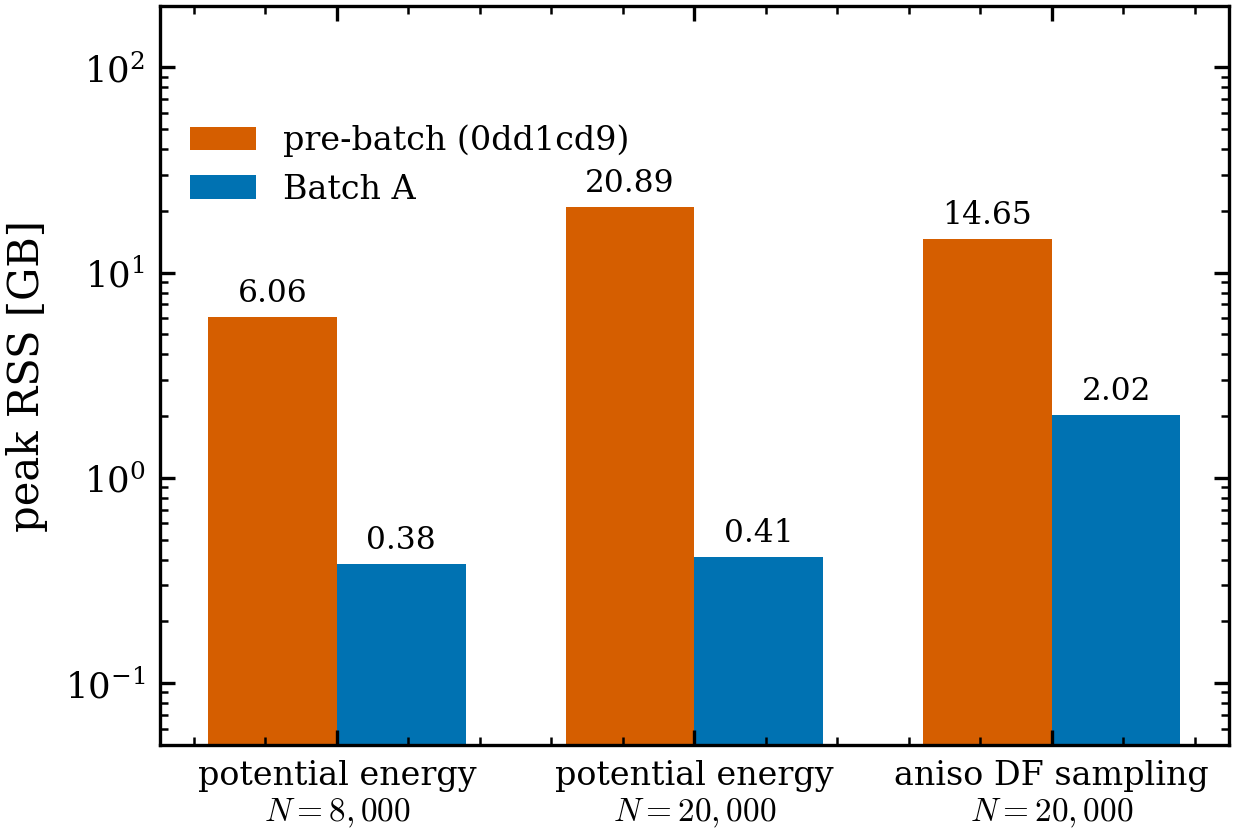
way; the blocked kernel is 0.41 GB at the same N. — Figure 1:Peak RSS (resident set size, GB; log scale) per kernel call, measured in isolated subprocesses (2026-06-10, `scripts/benchmark_batch_a.py`). The dense potential-energy kernel’s peak is macOS-memory-pressure dependent (20.9 GB in this run; 32.8 GB in the original probe) — decisively machine-filling either way; the blocked kernel is 0.41 GB at the same $N$ .

Kernel	$N$	pre-batch peak RSS	Batch A peak RSS
`compute_potential_energy`	8,000	6.06 GB	0.38 GB (16×)
`compute_potential_energy`	20,000	20.9 GB (32.8 GB in the original probe)	0.41 GB (≥ 50×)
aniso `LIMEPYVelocityDF.sample_velocities`	20,000	14.6 GB (10.9 GB in the original probe)	2.02 GB (≥ 5.4×; construction-dominated — see below)

The pass gates live in scripts/profile_cluster_memory.py (7 stages, including the $N = 10^5$ Engine A/B cluster samplers at 1.4–2.5 GB); the script exits nonzero on any gate regression, so this is a standing memory regression test, not a one-off measurement.

Why it was so large. The old energy kernel materialized all pairwise separations at once (positions[:,None,:] − positions[None,:,:], an $(N,N,3)$ float64 array — 9.6 GB at $N = 2\times10^4$ ) and, running eagerly, held several such intermediates simultaneously. The old anisotropic DF sampler evaluated a 256-point speed grid × ~91-term lowered-isothermal series per star under an eager vmap — a live $(N, 256, 91)$ block.

The fixes. (1) The virial kernels are now a jax.lax.scan over 256-row blocks — one $(256, N, 3)$ transient at a time — with the per-block computation wrapped in jax.checkpoint, so the gradient pass is also $O(\mathrm{block}\cdot N)$ (without rematerialization, the scan’s backward pass silently stores per-block residuals and rebuilds the $O(N^2)$ footprint; measured: jax.grad of the potential energy at $N=2\times10^4$ now peaks at 0.72 GB). Pair set and per-pair arithmetic are identical to the dense kernel — verified against an independent dense oracle at rtol 10^-13, gradient parity $\leq 2\times10^{-14}$ — only the float64 summation order changes across blocks. (2) The standalone DFs draw speeds from the same precomputed CDF tables the cluster sampler already used (~14 MB), cached on the module at construction and consumed through a jitted sampling core (eqx.filter_jit, the cluster/sampling.py pattern) so the draw chain fuses instead of materializing every eager intermediate. A staged profile (2026-06-10, $N=2\times10^4$ aniso) attributes the remaining footprint: construction dominates (~1.8 GB: two ODE solves + the $\mu$ integral + the cached table build, paid once per model), the jitted draw adds only +0.20 GB (eager it was +0.63 GB), and warm draws take 15 ms after the one-time ~0.5 s compile. The exact per-star quadrature is retained as the oracle behind speed_method="quadrature" (also jitted now). A further lax.map chunking of the table draw was evaluated and rejected on measurement: it would shave part of a 0.2 GB component inside a construction-dominated stage while adding scan overhead to a millisecond hot path.

Wall-clock: measured, including the honest small- $N$ crossover¶

Median wall-clock per call vs N (log–log; 2026-06-10). (a)
compute_potential_energy: the blocked kernel wins above N \approx 5{,}000
(2.4× at N=8{,}000: 0.169 → 0.070 s) and is the only feasible option at
N = 2\times10^4 (0.216 s); below the crossover the dense broadcast is
faster (0.013 vs 0.045 s at N=2{,}000) — scan overhead dominates when the
dense transient is only ~100 MB. (b) anisotropic LIMEPY sampling, after
the sampler-fusion follow-up (table cached at construction + jitted core):
warm draws cost 3–16 ms across N = 2\times10^3–2\times10^4 — 55×
faster than the pre-batch quadrature at N=10^4 (0.497 → 0.009 s) — with the
former small-N table-build penalty eliminated (the build moved into
construction, paid once per model; a ~0.5 s jit compile is paid on the first
draw per N). The quadrature oracle (green) also runs in the jitted core
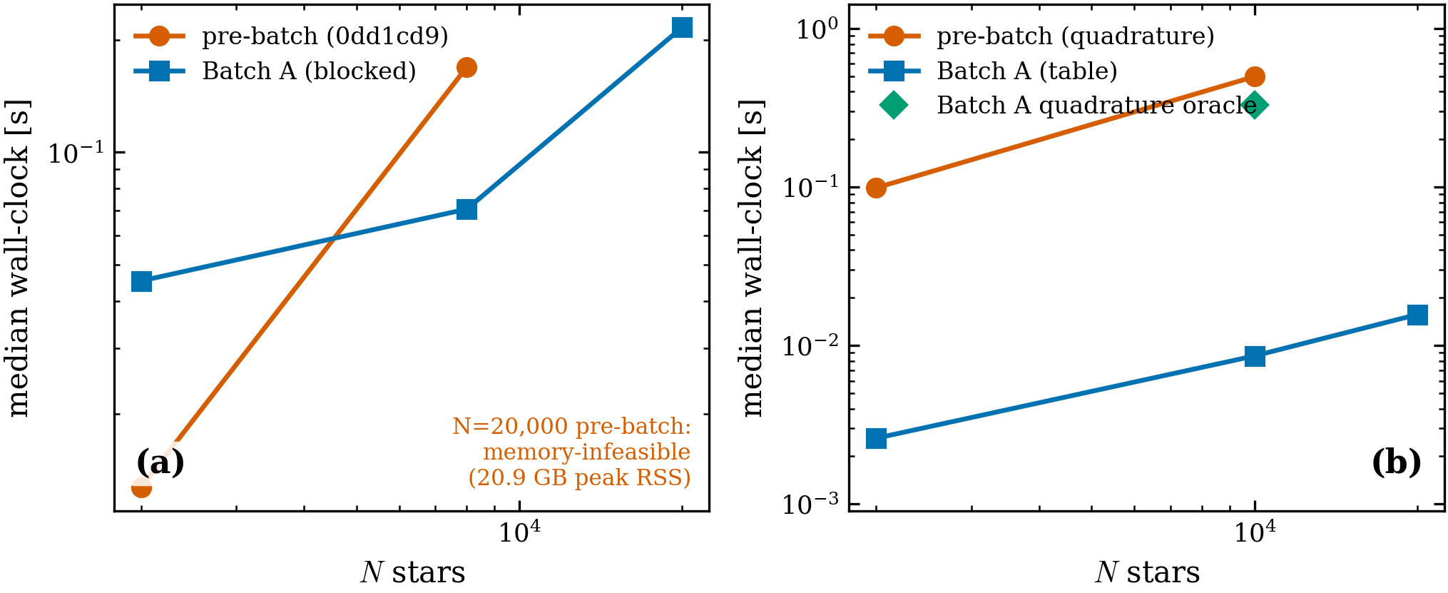
(0.33 s at N=10^4, lax.map-chunked to bound its memory). — Figure 2:Median wall-clock per call vs $N$ (log–log; 2026-06-10). **(a)** `compute_potential_energy`: the blocked kernel wins above $N \approx 5{,}000$ (2.4× at $N=8{,}000$ : 0.169 → 0.070 s) and is the only feasible option at $N = 2\times10^4$ (0.216 s); below the crossover the dense broadcast is faster (0.013 vs 0.045 s at $N=2{,}000$ ) — scan overhead dominates when the dense transient is only ~100 MB. **(b)** anisotropic LIMEPY sampling, after the sampler-fusion follow-up (table cached at construction + jitted core): warm draws cost **3–16 ms** across $N = 2\times10^3$ – $2\times10^4$ — 55× faster than the pre-batch quadrature at $N=10^4$ (0.497 → 0.009 s) — with the former small- $N$ table-build penalty eliminated (the build moved into construction, paid once per model; a ~0.5 s jit compile is paid on the first draw per $N$ ). The quadrature oracle (green) also runs in the jitted core (0.33 s at $N=10^4$ , `lax.map`-chunked to bound its memory).

Timings are reported, never gated (they vary with machine load); the memory ratios are gated (the benchmark requires ≥ 5× at $N=8{,}000$ , measures 16×).

Distribution fidelity of the table-routed draws¶

Routing the speed marginal through CDF tables must not change the physics. The angular conditional $\cos\theta\,|\,u$ stays exact; only the speed marginal is tabulated. The standing gates (unit suite, TableRouting classes): KS $D < 0.02$ , mean/second-moment ratios within 2%/3%, $\beta(r)$ preserved to 0.06. Measured (2026-06-10, $N = 2\times10^4$ per draw, scripts/validate_speed_routing.py, ALL PASS): King KS $D = 1\times10^{-4}$ , LIMEPY $3\times10^{-4}$ with $\max|\Delta\beta| = 1\times10^{-5}$ , Michie $6.7\times10^{-3}$ with $\max|\Delta\beta| = 0.042$ (King/LIMEPY draws are variate-paired with the oracle, hence near-exact; Michie’s $(u_t, u_r)$ oracle consumes keys in a different order, so its comparison is unpaired — the honest statistical case).

Anisotropic LIMEPY (W_0=5, g=1, r_a=4): (a) speed distribution,
table default vs exact quadrature oracle, N=2\times10^4; (b) measured
\beta(r) from the same draws — indistinguishable, as required (the angular
conditional is shared exactly). King and Michie versions of this figure are
embedded on the King and
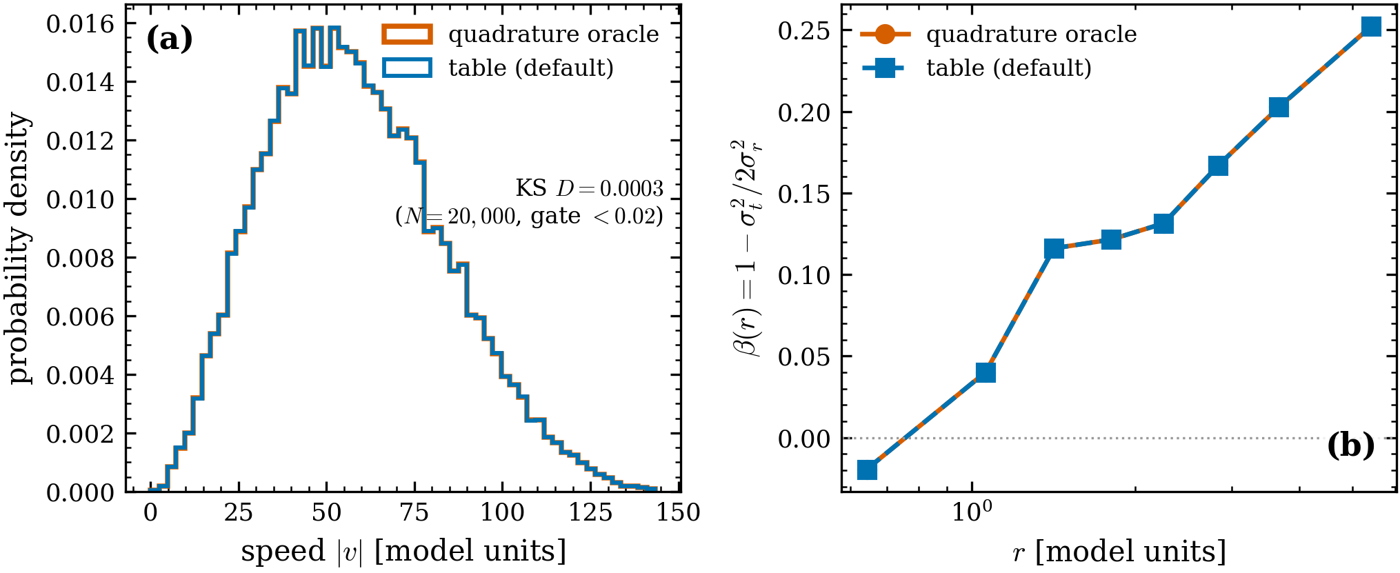
Michie pages. — Figure 3:Anisotropic LIMEPY ( $W_0=5$ , $g=1$ , $r_a=4$ ): (a) speed distribution, table default vs exact quadrature oracle, $N=2\times10^4$ ; (b) measured $\beta(r)$ from the same draws — indistinguishable, as required (the angular conditional is shared exactly). King and Michie versions of this figure are embedded on the King and Michie pages.

What this enables¶

Exact potential energies, virial diagnostics, and their jax.grad at $N \gtrsim 10^5$ on a laptop (footprint linear in $N$ ; block_size is tunable); standalone anisotropic DF sampling at survey scale with millisecond repeated draws (build the DF once, draw many times — e.g. seed ensembles); and a CI-able memory regression gate (the limepy_df_aniso gate is tightened to 2.5 GB to lock in the fusion win). The $N=2\times10^4$ virial workloads that previously OOM’d this 68.7 GB machine now fit in half a GB; the remaining DF-stage floor (~1.8 GB) is model construction (ODE solves + the $\mu$ integral), a future optimization target if it ever matters — it is paid once per model, not per draw.

Peak memory: before vs after¶

Wall-clock: measured, including the honest small-NNN crossover¶

Distribution fidelity of the table-routed draws¶

What this enables¶

Wall-clock: measured, including the honest small- $N$ crossover¶