EFF profile validation - progenax — differentiable initial conditions for N-body simulations

The EFF suite verifies the closed-form density, the inverse-CDF sampling, and the ergodic (Eddington) velocity DF. Test file: tests/validation/test_eff_physics.py (see the test dashboard for the live per-suite count); figures: scripts/validate_eff.py.

What is verified¶

Each row maps to assertions in test_eff_physics.py. The Tolerance is the exact bound the test enforces; the Measured value is regenerated by scripts/validate_eff.py (which prints expected-vs-measured for every figure).

Property	Tolerance (as tested)	Measured	Anchor
Density at scale radius $\rho(a)=\rho_0/2^{\gamma/2}$	10^-10 abs	0.2500 (γ=4)	closed-form density
Asymptotic slope $\rho\propto r^{-\gamma}$ ( $r\gg a$ )	$1\%$ rel	-3.97 (γ=4)	power-law limit
$\gamma=5$ reduces to Plummer	exact	max rel $=0.0$	$(1+r^2/a^2)^{-5/2}$
Tidal truncation ( $r\le r_t$ )	100%	100%	truncated sampling
Concentration increases with $\gamma$	monotone median $r$	$r_{1/2}=[15.8,6.3,2.2,1.3]$ (γ=2–5)	inverse-CDF sampling
Sampled CDF vs profile grid	max $\|\Delta\mathrm{CDF}\|<0.02$	$2.7\times10^{-3}$	inverse-CDF accuracy
Eddington $f(\mathcal{E})$ physical	$f\ge0$ , increasing	$\min f>0$ , monotone (γ=3,4,5)	ergodic DF non-negativity
Velocity isotropy $\langle v_x^2\rangle\!\approx\!\langle v_y^2\rangle\!\approx\!\langle v_z^2\rangle$	$<10\%$ rel spread	$0.3\%$	isotropic DF
Bound fraction ( $v\le v_{\rm esc}$ )	100%	100.00%	$v_{\rm esc}^2=2\kappa\Psi(r)$
Virial $Q=T/\|V\|$ (mild trunc, γ=5)	$\|Q-0.5\|<0.05$	0.502	Eddington equilibrium
Sampling differentiability ( $a,\gamma,M$ )	AD $=$ central-FD	rel err $5\!\times\!10^{-11}$ , $2\!\times\!10^{-11}$ , $2\!\times\!10^{-6}$	`jax.lax.scan` sampling

Figures¶

Generated by scripts/validate_eff.py (PASS/FAIL per panel; PNG + PDF vector).

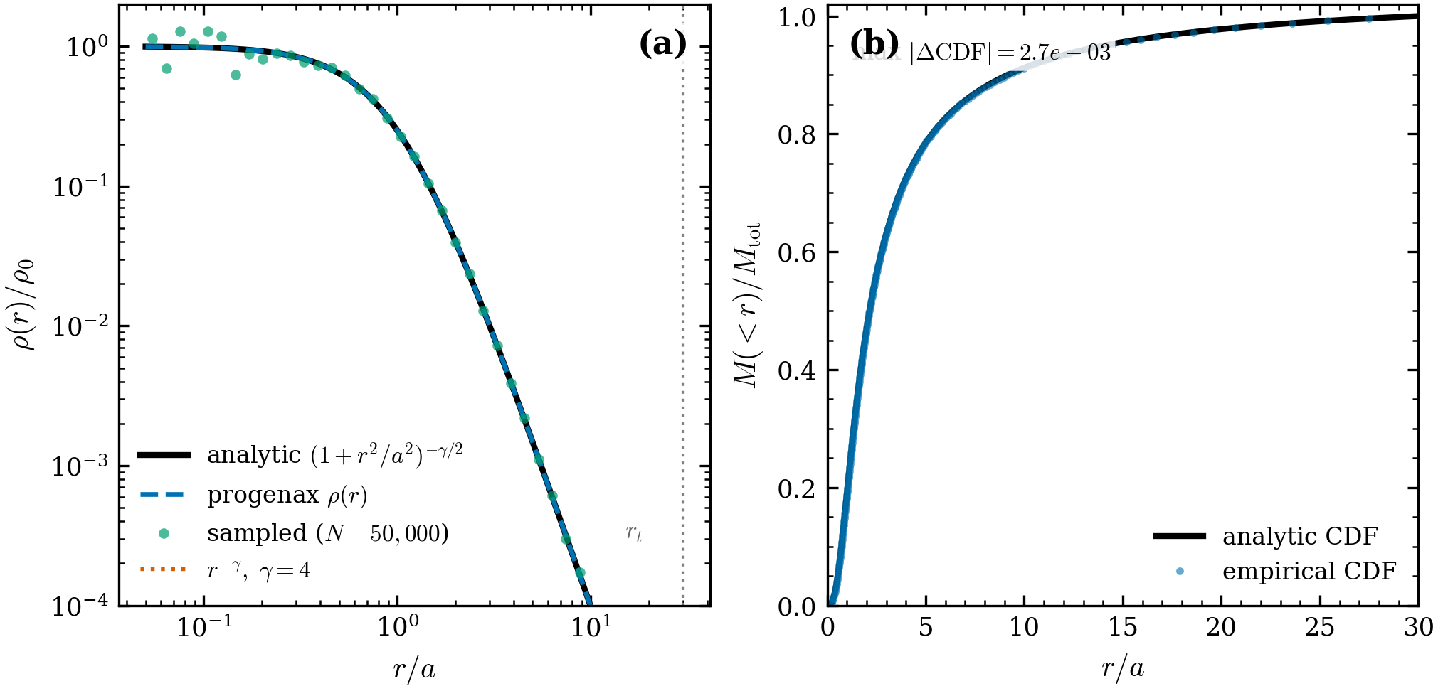
$Density, asymptotic slope, and truncation (γ=4). (a) EFFProfile.density (dashed) on the analytic (1+r^2/a^2)^{-\gamma/2} (solid) and the N=5\times10^4 sample; the recovered outer slope is -3.97 vs -\gamma=-4, and the profile terminates at r_t. (b) The empirical CDF matches the profile’s inverse-CDF grid to max |\Delta\mathrm{CDF}|=2.7\times10^{-3}.$

Figure 1:Density, asymptotic slope, and truncation (γ=4). (a) EFFProfile.density (dashed) on the analytic $(1+r^2/a^2)^{-\gamma/2}$ (solid) and the $N=5\times10^4$ sample; the recovered outer slope is -3.97 vs $-\gamma=-4$ , and the profile terminates at $r_t$ . (b) The empirical CDF matches the profile’s inverse-CDF grid to max $|\Delta\mathrm{CDF}|=2.7\times10^{-3}$ .

The γ family and the Plummer limit. Normalized density for \gamma=2,3,4,5:
larger \gamma is more centrally concentrated (median radius
15.8\to1.3\,a). The \gamma=5 curve coincides exactly with Plummer (dotted;
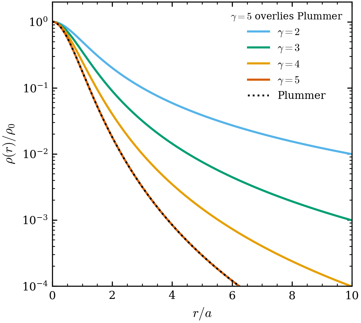
max rel =0), the analytic limit of the EFF family. — Figure 2:**The γ family and the Plummer limit.** Normalized density for $\gamma=2,3,4,5$ : larger $\gamma$ is more centrally concentrated (median radius $15.8\to1.3\,a$ ). The $\gamma=5$ curve **coincides exactly with Plummer** (dotted; max rel $=0$ ), the analytic limit of the EFF family.

Eddington velocity equilibrium. (a) Sampled \sigma_{1d}(r) with measured
isotropy 0.3\%. (b) Every velocity satisfies v\le v_{\rm esc}(r) — 100%
bound. (c) The mild-truncation (\gamma=5) IC sits at virial Q=0.502;
the sharp-truncation (\gamma=3) point at Q=0.46 shows the sub-virial caveat
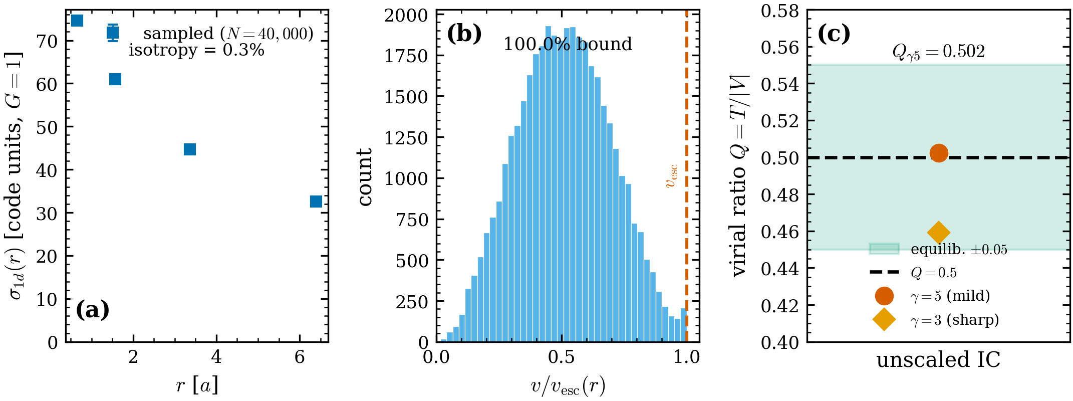
honestly. — Figure 3:**Eddington velocity equilibrium.** (a) Sampled $\sigma_{1d}(r)$ with measured isotropy $0.3\%$ . (b) Every velocity satisfies $v\le v_{\rm esc}(r)$ — **100% bound**. (c) The mild-truncation ( $\gamma=5$ ) IC sits at virial **$Q=0.502$** ; the sharp-truncation ( $\gamma=3$ ) point at $Q=0.46$ shows the sub-virial caveat honestly.

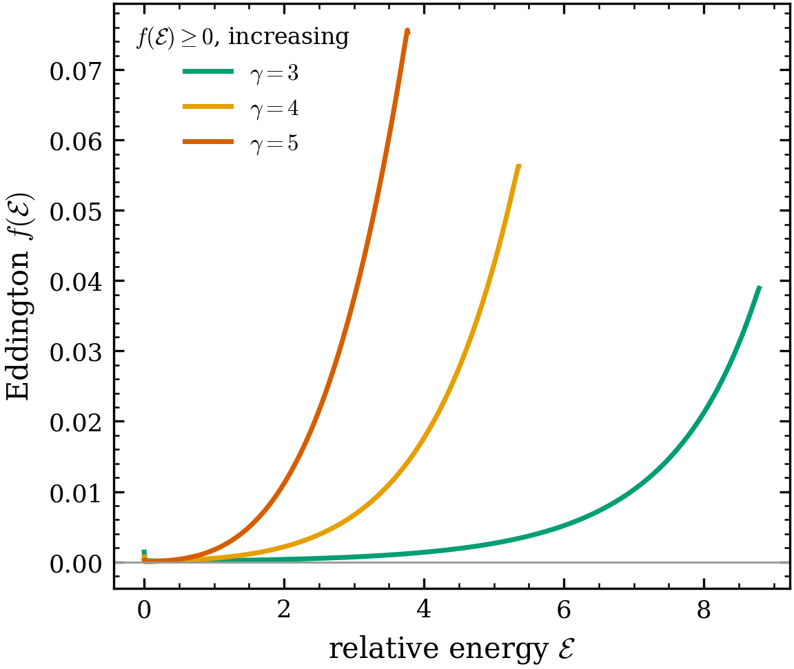
The ergodic DF is physical. The tabulated Eddington f(\mathcal{E}) is
non-negative and monotonically increasing in energy for \gamma=3,4,5 — the
conditions for a valid isotropic equilibrium DF. — Figure 4:**The ergodic DF is physical.** The tabulated Eddington $f(\mathcal{E})$ is non-negative and monotonically increasing in energy for $\gamma=3,4,5$ — the conditions for a valid isotropic equilibrium DF.

Differentiability¶

EFF’s structural parameters are differentiable, enabling gradient-based / HMC inference. In particular γ is a differentiable structural parameter — the EFF analogue of King’s $W_0$ (both are differentiable; see Differentiability).

Gradient validation (autodiff vs central finite difference). (a)
\partial\log\rho/\partial a, (b) \partial\rho/\partial\gamma, (c)
\partial\sqrt{\kappa}/\partial M_{\rm tot} (the velocity scale): autodiff (line)
and finite difference (circles) agree to max rel err 5\times10^{-11},
2\times10^{-11}, 2\times10^{-6}, so (a,\gamma,M_{\rm tot}) can be inferred
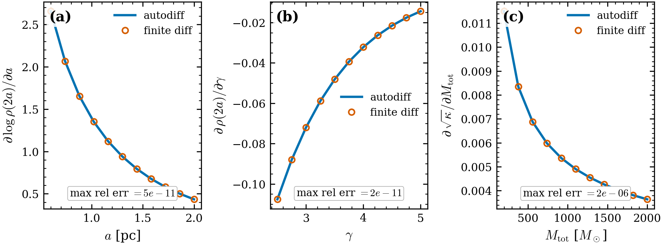
jointly. — Figure 5:**Gradient validation (autodiff vs central finite difference).** (a) $\partial\log\rho/\partial a$ , (b) $\partial\rho/\partial\gamma$ , (c) $\partial\sqrt{\kappa}/\partial M_{\rm tot}$ (the velocity scale): autodiff (line) and finite difference (circles) agree to **max rel err $5\times10^{-11}$ , $2\times10^{-11}$ , $2\times10^{-6}$** , so $(a,\gamma,M_{\rm tot})$ can be inferred jointly.

How to run¶

# physics tests (~9 s on CPU)
pytest tests/validation/test_eff_physics.py -q

# regenerate the five figures with PASS/FAIL tables
python scripts/validate_eff.py

What this suite does not test¶

Radial anisotropy — the isotropic Eddington DF is covered; Osipkov–Merritt anisotropy is available via EFFVelocityDF(anisotropy_radius=...) and validated with the Michie model.
Multi-mass / unified lowered models — see the lowered-model-family roadmap.

References¶

Elson et al. (1987) is the original (note the surface-vs-3-D slope convention above). Theory at EFF profile.

References¶

Elson, R. A. W., Fall, S. M., & Freeman, K. C. (1987). The structure of young star clusters in the Large Magellanic Cloud. The Astrophysical Journal, 323, 54–78. 10.1086/165807