The King velocity DF is the lowered-Maxwellian that defines the King spatial profile in the first place. Unlike Plummer — where the DF follows from the density profile via Eddington inversion — King’s DF is the input, and the density profile follows from integrating the DF over velocity space (King profile). Sampling King velocities is therefore conceptually simpler than sampling Plummer velocities: at each particle’s position, draw from the truncated Maxwellian directly.
The lowered-Maxwellian DF
For a particle of specific energy at position , the King DF is
where is the central one-dimensional velocity dispersion, is the potential at the tidal radius, and is a normalisation constant. The “-1” subtraction is the lowering: it ensures the DF vanishes at rather than extending exponentially to as a pure Maxwellian would.
In terms of the dimensionless central potential (King profile, (1)), the DF becomes
at any radius where the local dimensionless potential is . The escape speed at the tidal radius is zero (, ), so no particles populate that boundary — the cluster is sharply truncated.
Marginal speed distribution
Integrating the DF over velocity directions gives the speed distribution at fixed position:
The prefactor is the spherical-shell volume element in velocity space. The bracketed factor is positive throughout and zero at the upper bound — which means inverse-CDF sampling on produces velocities in with no rejection.
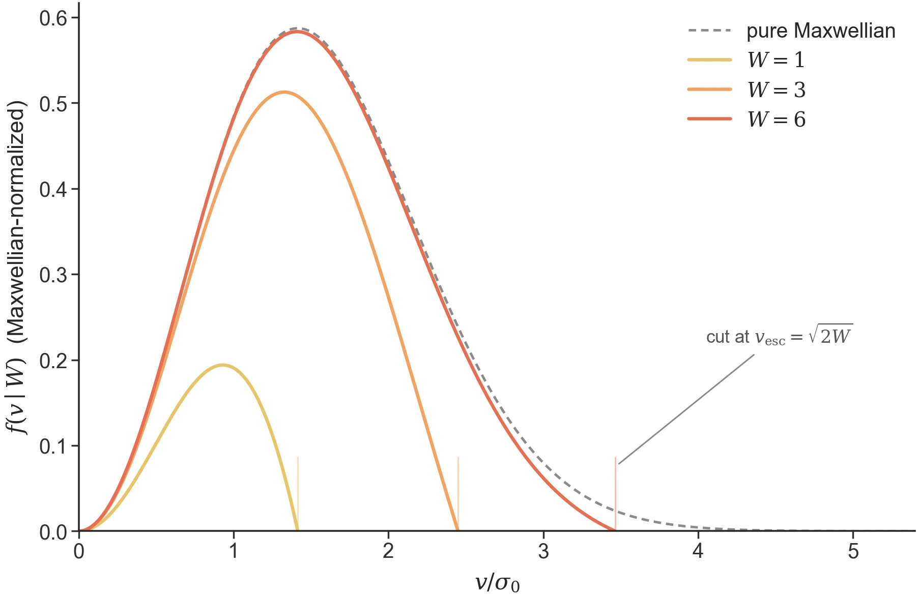
Figure 1:What “lowering” means. One normalized Maxwellian (grey, dashed) and the King
speed distribution at three local well depths: at (a cluster core)
the truncation barely bites, at (near the tidal edge) most of the
Maxwellian is cut away. The lowering matters most where the well is
shallow — the origin of King clusters’ cold outskirts. Regenerate:
python -m laboratory.icviz --only king-lowered-maxwellian.
Sampling
progenax samples King velocities via a per-particle inverse-CDF on (3):
# At each particle's radius r, look up W(r) from the King ODE solution
W_per_particle = jnp.interp(radii / r_c, xi_grid, psi_grid, left=W0, right=0.0)

# Per particle: build a 1-D speed CDF on [0, sqrt(2W)] and invert it (vmap'd)
def sample_unit_speed(key, W):
    u_grid = jnp.linspace(0.0, jnp.sqrt(2.0 * W), N_SPEED_GRID)   # 256 points
    g = u_grid**2 * (jnp.exp(W - u_grid**2 / 2.0) - 1.0)         # eq:king-fv
    cdf = jnp.cumsum(0.5 * (g[1:] + g[:-1])) * du                # trapezoid
    return jnp.interp(jax.random.uniform(key), cdf / cdf[-1], u_grid)

u = jax.vmap(sample_unit_speed)(keys, W_per_particle)            # speed / sigma_0
v_vec = (sigma_0 * u)[:, None] * isotropic_unit_vector(key2, N)
Each particle builds its own fixed-size (256-point) speed grid scaled
to its local escape speed and inverts the trapezoidal
CDF by interpolation — there is no precomputed cross- table. The grid
size is fixed and the operations are jnp.interp/vmap only (no
while_loop), so the whole pipeline is JIT-compatible and differentiable
in via the chain .
Velocity dispersion profile
The King DF’s velocity dispersion at radius is
(in units where ). The integrals do not have closed
form in general, but progenax precomputes on the same
-grid used for the speed-CDF table inside the sampler. The current
public KingVelocityDF API exposes sample_velocities; it does not
export a separate velocity-dispersion method. The dispersion is
monotonically increasing in : as and
as (the untruncated-Maxwellian
limit). Since decreases outward — from at the centre to 0 at
the tidal radius — falls with radius and vanishes at the tidal
boundary, where the escape speed . King clusters therefore have
cold outskirts, in contrast to a Plummer sphere whose dispersion also
declines outward but stays finite at all radii.
Check yourself
1. Which is most Maxwellian?
Before studying Figure 1: does the King DF resemble a Maxwellian most at the cluster centre or the edge? (Centre: large pushes far into the Maxwellian tail, so almost nothing is cut.)
2. Quantify the cut
Compute the fraction of a pure Maxwellian beyond : . At that is 0.57 — the lowering removes the majority of the distribution — while at it is 0.007. Check both against the figure by eye, then verify with a quick quadrature of .
Pairing with the King profile
The King DF is in equilibrium with the King density profile by construction: both are derived from the same lowered-isothermal Maxwellian. Pair them by using the same King concentration and tidal radius:
from progenax.profiles import KingProfile
from progenax.kinematics import KingVelocityDF
from jaxstro.units import STELLAR

profile = KingProfile.from_W0_rc(W0=7.0, r_c=1.0)
df = KingVelocityDF(W0=7.0, r_c=1.0)   # r_t is derived from W0 internally

masses = jnp.ones(1000)
positions = profile.sample_positions(masses, key_pos)
velocities = df.sample_velocities(positions, masses, key_vel, G=STELLAR.G)
KingVelocityDF takes only (W0, r_c) — it re-solves the King ODE
internally and derives the tidal radius from , so there is no
r_t argument. Using the same W0 and r_c in the profile and DF
keeps them consistent. Pairing a King profile at with a King DF
at would produce a mismatched non-equilibrium IC.
Differentiability
The King velocity DF is differentiable in (via ) and in the
total mass (). It is also
differentiable in : diffrax propagates
through the ODE solve, so the dispersion profile and other shape observables
carry correct gradients (gradient-validated in
King profile validation). The lone non-differentiable quantity
is the scalar tidal radius , whose -derivative is zeroed by the
argmax zero-crossing in _find_tidal_radius; inference should therefore use
the profile shape rather than the scalar .
Consequently progenax supports joint gradient-based / HMC inference of the King structural parameters directly — e.g. fitting a cluster’s number-density and velocity-dispersion profiles. The lowered-model family formalized by Gieles & Zocchi (2015) (where the truncation parameter enters analytically) remains the natural extension for multi-mass / anisotropic generalisations; progenax plans to implement this family natively as its own differentiable generalization (see The differentiable lowered-model family (Engine A)), but it is not yet available.
Domain of validity
Single-mass equilibrium. Multi-mass equilibrium is described by the lowered-model family formalized by Gieles & Zocchi (2015), not by the standard King DF here.
Spherical and isotropic by default. Anisotropic and rotating variants live in Anisotropy and rotation.
Tidal cutoff is sharp. Real clusters have a smooth transition from the bound population to the tidal tail; King’s mathematical cutoff at is an idealisation. For studies where the tidal-tail kinematics matter, post-evolution analysis is the right approach.
Implementation, validation & references
In code:
src/progenax/kinematics/king_df.py(the per-particle lowered-Maxwellian speed sampler; the King ODE solve it shares with the profile is insrc/progenax/profiles/king.py) — see theKingVelocityDFAPI.Validated in: King profile — the regression suite that locks the true-DF equilibrium ( unscaled) and the gradients.
Primary sources: the lowered-isothermal model is King (1966); the multi-mass LIMEPY generalisation is Gieles & Zocchi (2015), and the
diffraxintegration follows the standard Aarseth et al. (1974) numerical prescription — full notes in the bibliography.
- Gieles, M., & Zocchi, A. (2015). A family of lowered isothermal models. Monthly Notices of the Royal Astronomical Society, 454, 576–592. 10.1093/mnras/stv1848
- King, I. R. (1966). The structure of star clusters. III. Some simple dynamical models. The Astronomical Journal, 71, 64–75. 10.1086/109857
- Aarseth, S. J., Henon, M., & Wielen, R. (1974). A comparison of numerical methods for the study of star cluster dynamics. Astronomy and Astrophysics, 37, 183–187.