Multi-mass LIMEPY equilibrium (Engine A) - progenax — differentiable initial conditions for N-body simulations

Engine A (MultiComponentCluster.from_components / .from_mass_segregation / .from_imf) is progenax’s differentiable multi-component lowered-isothermal family (Gieles & Zocchi (2015), §2.2): every component $j$ shares ONE self-consistent potential solved from the coupled Poisson equation, with a single free scale per component — the velocity-scale ratio $w_j = s_j/s$ (mass segregation is $w_j = \mu_j^{-\delta}$ ). Heavier components are more centrally concentrated as an equilibrium property, not an imposed reshuffle — the contrast with the primordial generator on the mass-segregation page. Test files: tests/validation/test_multimass_equilibrium_physics.py plus the DF-table unit suites (tests/unit/profiles/test_limepy_tables.py; table threading in tests/unit/profiles/test_limepy_multimass.py) — see the test dashboard for the live per-suite counts. Figures + PASS/FAIL: scripts/validate_multimass_equilibrium.py, scripts/validate_multimass_anisotropy.py, scripts/validate_df_tables.py.

What is verified — isotropic equilibrium¶

Each row maps to assertions in test_multimass_equilibrium_physics.py; Measured values are from the 2026-06-10 run of scripts/validate_multimass_equilibrium.py (two-component model, $W_0=7$ , $g=1$ , $m_j = [1, 4]\,M_\odot$ , ALL PASS) unless noted.

Property	Tolerance (as tested)	Measured	Anchor
Theoretical per-component $Q_j$ (mean-field, no sampling)	$\|Q_j - 0.5\| < 2\times10^{-3}$ , all $\delta$	0.5001–0.5002 (both components, $\delta \in [0, 0.6]$ )	exact-quadrature virial oracle — the rigorous “each mass group is in equilibrium” statement
Sampled global $Q = T/\|V\|$ , unscaled	$\|Q - 0.5\| < 0.03$ ( $\delta \in \{0, 0.3, 0.6\}$ )	0.497–0.500 (5 seeds $\times$ 8000)	$2T + V = 0$
Per-component $\sigma_{1d,j}(r)$ vs analytic LIMEPY moment $s_j\sqrt{I_2/3I_0}$	rel $< 7\%$ per component (core bin, $N=40$ k)	$< 1\%$ across resolved bins (figure panel b)	each component drawn from ITS OWN equilibrium DF
Sampled per-group $Q_j$ (light, $N$ -body observable, softening $=0$ )	$\|Q - 0.5\| < 0.04$	0.496–0.497 across $\delta$	finite- $N$ estimator of the exact 0.5
Sampled per-group $Q_j$ (heavy)	$\|Q - 0.5\| < 0.06$ ( $\delta \le 0.5$ )	$0.503 \to 0.534$ as $\delta: 0 \to 0.6$	documented finite- $N$ positive bias (see note)
$\delta = 0$ is the single-mass model; segregation grows with $\delta$	ratio $= 1 \pm 10^{-2}$ at 0, strictly monotone	$r_{h,\rm light}/r_{h,\rm heavy}: 1.0 \to 2.6$ over $\delta \in [0, 0.6]$	controlled equipartition knob

Multi-mass equilibrium summary (scripts/validate_multimass_equilibrium.py,
PASS). (a) Per-component density profiles: the heavy component is more
centrally concentrated — segregation built in as an equilibrium. (b) Sampled
\sigma_{1d,j}(r) (points) on the analytic LIMEPY moment (lines) for both
components — the proof each mass group is drawn from its own equilibrium DF
(agreement <1\%). (c) Segregation strength
r_{h,\rm light}/r_{h,\rm heavy} vs \delta: 1.0 at \delta=0, rising
monotonically to 2.6 at \delta=0.6. (d) Per-group virial: theory Q_j
flat at 0.5 (thick faint lines); sampled light + global tight on 0.5; the
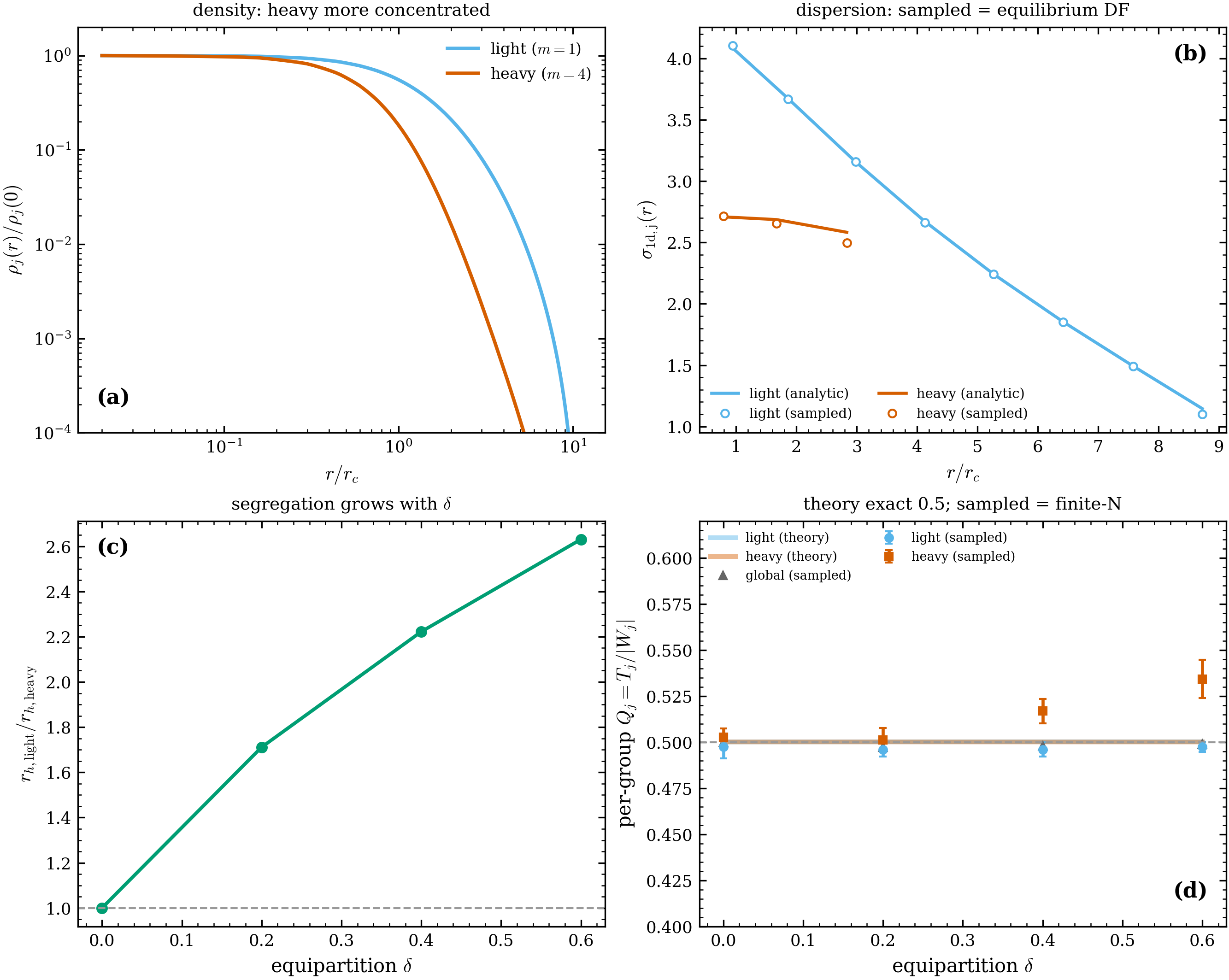
heavy component’s positive finite-N offset grows with \delta. — Figure 1:**Multi-mass equilibrium summary** (`scripts/validate_multimass_equilibrium.py`, PASS). (a) Per-component density profiles: the heavy component is more centrally concentrated — segregation built in as an equilibrium. (b) Sampled $\sigma_{1d,j}(r)$ (points) on the analytic LIMEPY moment (lines) for both components — the proof each mass group is drawn from its own equilibrium DF (agreement $<1\%$ ). (c) Segregation strength $r_{h,\rm light}/r_{h,\rm heavy}$ vs $\delta$ : 1.0 at $\delta=0$ , rising monotonically to 2.6 at $\delta=0.6$ . (d) Per-group virial: theory $Q_j$ flat at 0.5 (thick faint lines); sampled light + global tight on 0.5; the heavy component’s positive finite- $N$ offset grows with $\delta$ .

What is verified — anisotropic sampler¶

With a finite anisotropy radius, each component’s DF is the Michie/Osipkov-Merritt LIMEPY form $f(E, J^2) \propto e^{-J^2/2r_{a,j}^2 s_j^2}\,E_\gamma(g, (\phi_t - E)/s_j^2)$ , $r_{a,j} = r_a\,\mu_j^\eta$ . The sampler must carry the right anisotropy, not merely “some”: sampled $\beta_j(r) = 1 - \sigma_t^2/2\sigma_r^2$ is gated against the DF’s own $(u, c)$ -quadrature $\beta$ — including the LIMEPY signature rise to a radial-bias peak near $\sim 0.5\,r_t$ and turnover toward $r_t$ (truncation removes the most radial orbits at the edge). Measured values from the 2026-06-10 run of scripts/validate_multimass_anisotropy.py ( $r_a = 5$ , $\eta = 0$ , $\delta = 0.4$ , ALL PASS).

Property	Tolerance (as tested)	Measured	Anchor
Sampled $\beta_{\rm light}(r)$ vs DF quadrature (resolved bins, $r \le 0.8\,r_t$ )	$\|\Delta\beta\| < 0.04$ per bin, seed-averaged (8 bins checked)	all 8 bins pass; e.g. $0.218 \pm 0.003$ vs DF 0.219 at $0.46\,r_t$ (8 seeds $\times$ 60k)	the DF’s own 2nd moments — rise + truncation turnover reproduced
$\beta$ peak location/height	(shape, not gated separately)	peak $\approx 0.23$ near $0.55\,r_t$ , turning over toward $r_t$	LIMEPY truncation signature
Edge bins ( $r \gtrsim 0.8\,r_t$ ): ratio-noise convergence	not gated (plotted with errors); convergence study	16-seed average over 0.65– $0.75\,r_t$ : $0.191 \pm 0.012$ vs DF 0.193	$\beta$ is a ratio statistic; $\langle v_r^2\rangle \to 0$ at the edge, so single-seed $\beta$ is noise-dominated — it converges to the DF under seed-averaging
Global $Q$ (anisotropic), unscaled	$\|Q - 0.5\| < 0.04$ , all $\delta$	0.495–0.501 over $\delta \in [0, 0.6]$ (4 seeds $\times$ 20k)	the scalar virial theorem is anisotropy-blind

Anisotropic sampler validation (scripts/validate_multimass_anisotropy.py,
PASS). (a) Seed-averaged sampled \beta_j(r) (\pm sem, 8 seeds \times
60k) on the DF’s own quadrature \beta for both components — the rise to the
radial-bias peak and the truncation turnover are both reproduced; the
outermost bin shows the honest ratio-noise error bar. (b) \sigma_r(r) and
\sigma_t(r) separately, sampled vs DF: \sigma_r > \sigma_t in the bias
region — the kinematic content of \beta > 0. (c) Global Q vs \delta for
anisotropic models: 0.5 with no rescale. (d) Analytic
\beta_{\rm light}(r) for r_a = 8, 6, 5, 4: the anisotropy is a controlled
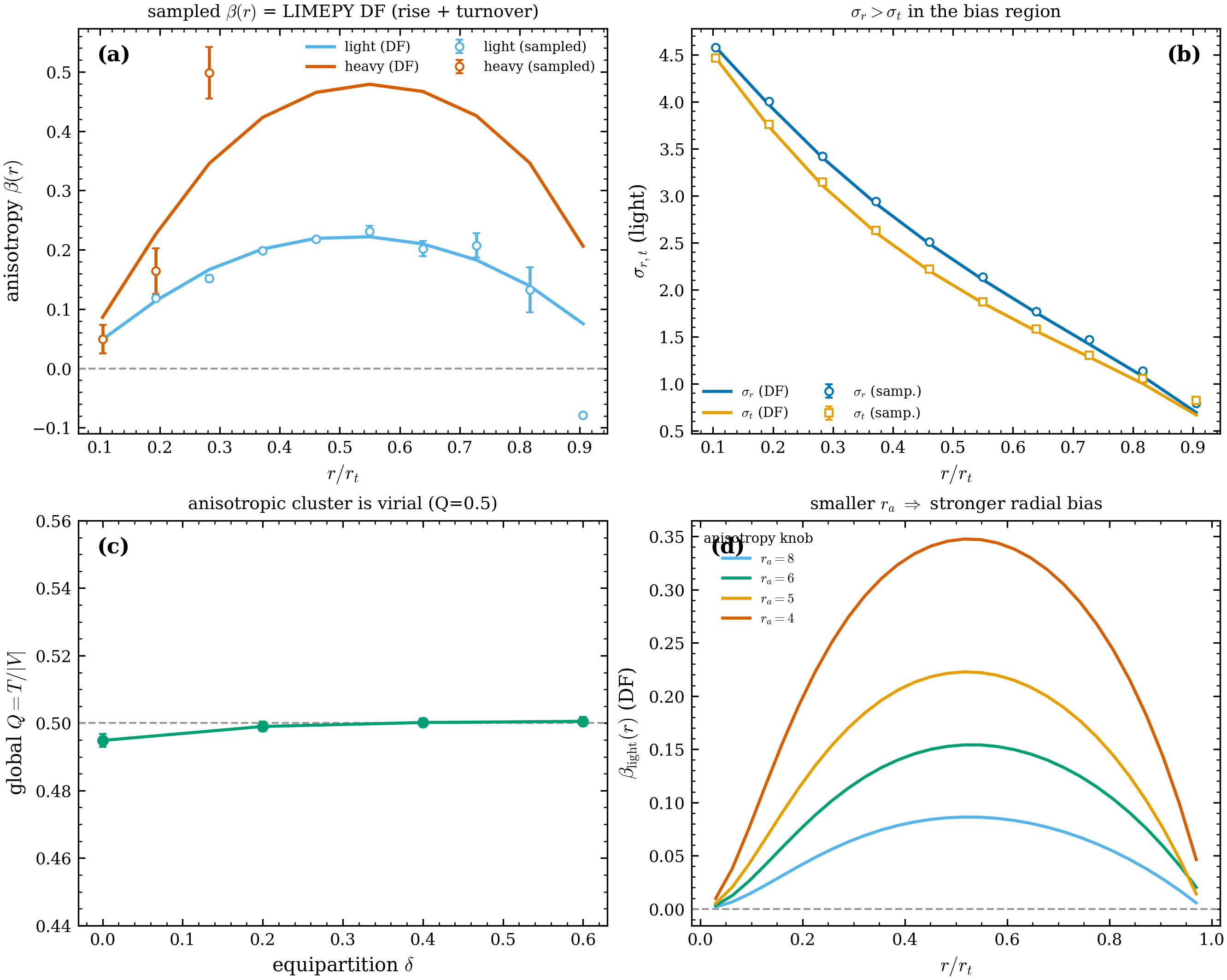
knob (smaller r_a \Rightarrow stronger radial bias). — Figure 2:**Anisotropic sampler validation** (`scripts/validate_multimass_anisotropy.py`, PASS). (a) Seed-averaged sampled $\beta_j(r)$ (± sem, 8 seeds $\times$ 60k) on the DF’s own quadrature $\beta$ for both components — the rise to the radial-bias peak and the truncation turnover are both reproduced; the outermost bin shows the honest ratio-noise error bar. (b) $\sigma_r(r)$ and $\sigma_t(r)$ separately, sampled vs DF: $\sigma_r > \sigma_t$ in the bias region — the kinematic content of $\beta > 0$ . (c) Global $Q$ vs $\delta$ for anisotropic models: 0.5 with no rescale. (d) Analytic $\beta_{\rm light}(r)$ for $r_a = 8, 6, 5, 4$ : the anisotropy is a controlled knob (smaller $r_a$ $\Rightarrow$ stronger radial bias).

DF tables — the accelerated path is budget-asserted against its oracle¶

Phase 1.5 replaced pointwise quadrature in the coupled-Poisson RHS and both sampler branches with three differentiable table primitives (profiles/limepy_tables.py): AnisoDensityTable (cubic-Lagrange on a $(\sqrt W, \operatorname{asinh} p)$ grid), SpeedCDFTable ( $256\times256$ isotropic inverse speed CDF, gated to $g \in [0, 3.5]$ ), and AnisoSpeedCDFTable ( $192\times48\times192$ speed marginal — the angular conditional $(\cos\theta \mid u, p)$ stays exact). The exact quadrature survives as a selectable oracle (aniso_method="quadrature"), so every budget below is a one-line regression test:

Quantity	Measured	Budget
Density $\hat\rho(W, p)$ table vs quadrature oracle ( $512\times96$ grid)	$6.05\times10^{-6}$	10^-5
Coupled solve $\|\psi_{\rm table} - \psi_{\rm quad}\|$ , 3 configs ( $W_0 = 5, 7, 9$ )	$\le 1.93\times10^{-4}$	$10^{-4}\,W_0$ each
Mass CDF	$4.5\times10^{-5}$	$5\times10^{-4}$
Iso / aniso speed moments vs DF quadrature	$\le 0.28\%$ / $\le 1.5\%$	statistical gates
$\beta(r)$ vs the DF’s own quadrature $\beta$	$< 0.06$ (unchanged by the tables)	$< 0.06$
$Q_j$ of a table-built model vs the quadrature oracle	$0.5001 \pm 1.5\times10^{-4}$	0.5
AD vs central-FD gradient through the table solve ( $w_j$ , $r_a$ )	$2.15\times10^{-4}$	rtol 10^-3
Table-AD vs quadrature-AD (FD-free cross-check)	$2.1\times10^{-4}$	report

Oracle independence: component_virial_ratios is deliberately quadrature-only — the equilibrium oracle must not share the approximation it checks. The table-built model proving $Q_j = 0.5001 \pm 1.5\times10^{-4}$ against that independent oracle is the end-to-end closure.

Performance (warm, measured at close-out): anisotropic construction $957 \to 170$ ms (5.6×); sampling at $N = 10^5$ : isotropic 67× ( $0.48\,\mu$ s/star), anisotropic 21.7× ( $2.9\,\mu$ s/star). The anisotropic table build dominates at small $N$ — break-even $\approx 3$ k stars (documented; below that, use the quadrature path).

Memory is bounded alongside speed: the $O(N^2)$ virial kernels run in fixed-size blocks with rematerialization (forward and gradient $O(\mathrm{block}\cdot N)$ ), and the standalone DFs route through the same tables. Measured peak RSS (scripts/profile_cluster_memory.py, all stages PASS):

Stage	$N$	Peak RSS
`import progenax`	—	0.19 GB
Engine A build + sample, isotropic	10⁵	1.4 GB
Engine A build + sample, anisotropic (OM)	10⁵	2.2 GB
Engine B halo+core build + sample	10⁵	2.5 GB
Virial / potential-energy kernel	$2\times10^4$	0.41 GB
Per-group virial oracle	$2\times10^4$	0.60 GB
Standalone anisotropic LIMEPY DF sampling	$2\times10^4$	2.3 GB

DF-table validation (scripts/validate_df_tables.py, ALL PASS).
(a) Pointwise density error vs the quadrature oracle: the 512\times96 grid
sits under the 10^{-5} budget (max 6.05\times10^{-6}); the coarser
160\times40 in-solve grid is reported honestly (it is sized to the solve
budget, not the pointwise one). (b) |\psi_{\rm table} - \psi_{\rm quad}|
for the three solve configs, each under its 10^{-4} W_0 budget (dashed).
(c) Warm wall times: solve and construction speedups with the shared table.
(d) AD vs central-FD gradient bars in (w_1, w_2, \hat r_{a,1}, \hat r_{a,2}),
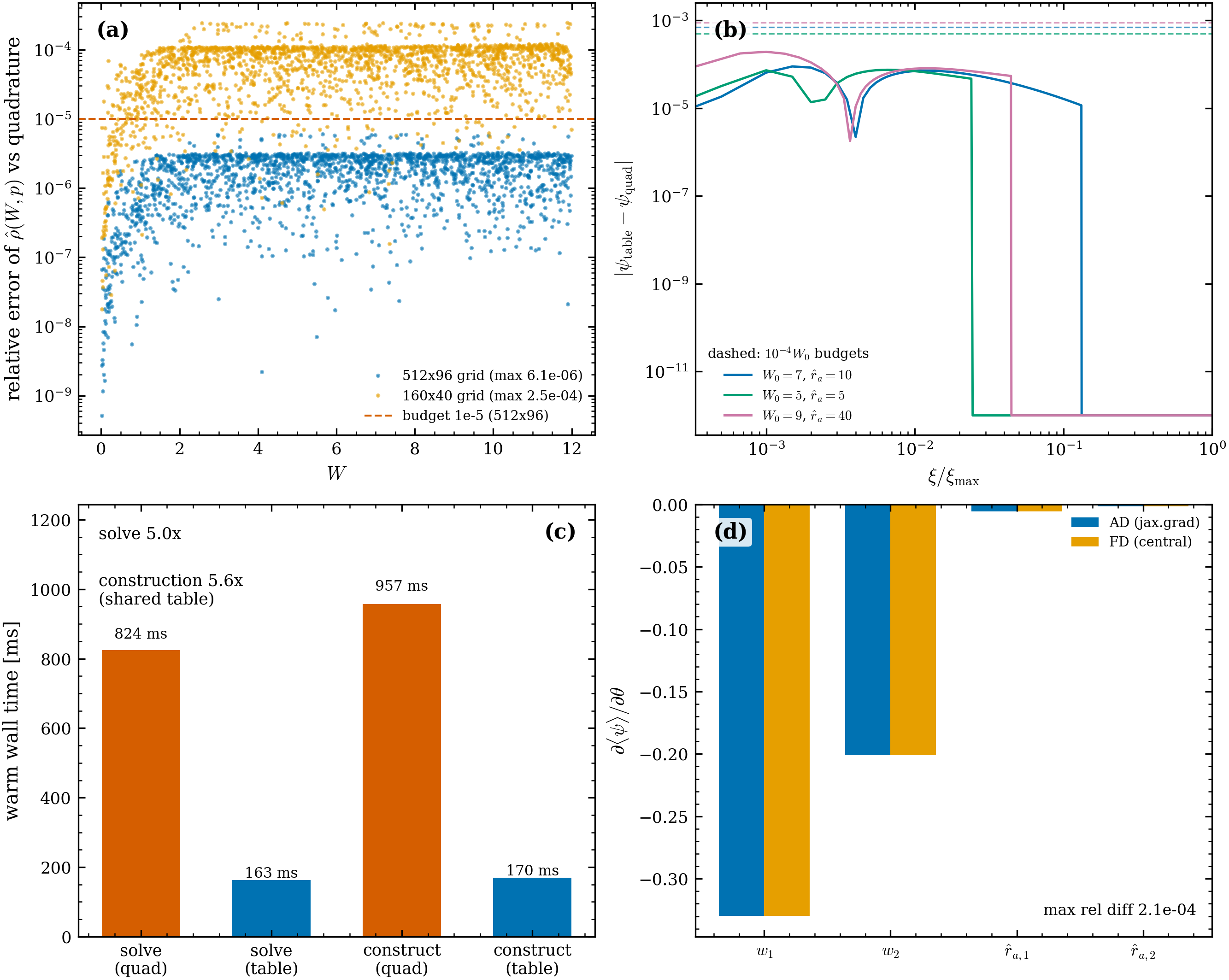
max rel diff 2.15\times10^{-4}. — Figure 3:**DF-table validation** (`scripts/validate_df_tables.py`, ALL PASS). (a) Pointwise density error vs the quadrature oracle: the $512\times96$ grid sits under the 10^-5 budget (max $6.05\times10^{-6}$ ); the coarser $160\times40$ in-solve grid is reported honestly (it is sized to the *solve* budget, not the pointwise one). (b) $|\psi_{\rm table} - \psi_{\rm quad}|$ for the three solve configs, each under its $10^{-4} W_0$ budget (dashed). (c) Warm wall times: solve and construction speedups with the shared table. (d) AD vs central-FD gradient bars in $(w_1, w_2, \hat r_{a,1}, \hat r_{a,2})$ , max rel diff $2.15\times10^{-4}$ .

Differentiability¶

The whole Engine A pipeline — coupled Poisson solve (table RHS included), mass CDF, and jax.lax.scan sampling — is differentiable in the structural parameters $(w_j, r_a, \delta, W_0, \ldots)$ : AD matches central FD through the table-backed solve to $2.15\times10^{-4}$ , and the table-path AD matches the quadrature-path AD (an FD-free check) to $2.1\times10^{-4}$ . A review-caught $W \le 0$ NaN-gradient bug at the truncation boundary (the $\sqrt{W}$ cotangent under jax.grad, masked only in the primal by where) was fixed pre-merge and is regression-tested.

How to run¶

# physics tests (6 validation tests; marked slow — each samples >= 8000 stars)
pytest tests/validation/test_multimass_equilibrium_physics.py -q

# DF-table unit suites (budgets + threading)
pytest tests/unit/profiles/test_limepy_tables.py tests/unit/profiles/test_limepy_multimass.py -q

# regenerate the figures with printed PASS/FAIL tables
env -u VIRTUAL_ENV uv run --no-sync python scripts/validate_multimass_equilibrium.py
env -u VIRTUAL_ENV uv run --no-sync python scripts/validate_multimass_anisotropy.py
env -u VIRTUAL_ENV uv run --no-sync python scripts/validate_df_tables.py

What this suite does not test¶

No N-body integration of the ICs — equilibrium is established by the exact-quadrature virial oracle, DF-moment matches, and the sampled estimators on the initial conditions, not by evolving them.
$\delta > 0.6$ — the model family approaches the Spitzer-unstable $\delta \to 1$ limit; the sampled heavy-group gate covers $\delta \le 0.5$ and the theory oracle $\delta \le 0.6$ only.
The outermost anisotropy bin ( $r \gtrsim 0.8\,r_t$ ) is plotted with its error bar but not gated — it is finite- $N$ ratio noise, shown converging to the DF under seed-averaging, not asserted per-seed.
Small- $N$ anisotropic table efficiency — below the $\approx 3$ k-star break-even the table build dominates; correctness is unaffected (budgets hold at all $N$ ), only speed.

References¶

Gieles & Zocchi (2015) (the multimass lowered-isothermal family; per-paper note in the bibliography, including the App. B density index and the 2018 erratum). The density-defined companion engine is validated at Multi-component Eddington equilibria (Engine B); the primordial (non-equilibrium) segregation generator at Mass segregation validation. This validation backs the multimass LIMEPY-equilibrium and DF-tables close-out.

References¶

Gieles, M., & Zocchi, A. (2015). A family of lowered isothermal models. Monthly Notices of the Royal Astronomical Society, 454, 576–592. 10.1093/mnras/stv1848