Michie-King anisotropy validation - progenax — differentiable initial conditions for N-body simulations

The Michie (1963) radial-anisotropy term on King’s (1966) lowered cutoff: a self-consistent, radially anisotropic cluster model. Test file: tests/validation/test_michie_physics.py (see the test dashboard for the live per-suite count); figures: scripts/validate_michie.py. Theory at Michie-King anisotropic model.

What is verified¶

Each row maps to assertions in test_michie_physics.py. Measured values are regenerated by scripts/validate_michie.py. All use $W_0=7$ , $r_c=1$ , with $r_a=8\,r_c$ for the anisotropic case (it truncates: $r_t/r_c\simeq56$ ) and $r_a=10^4\,r_c$ for the isotropic limit.

Property	Tolerance (as tested)	Measured	Anchor
Isotropic limit: $\rho_{\rm Michie}(r_a\!\to\!\infty)=\rho_{\rm King}$	10^-2 max rel	$2.7\times10^{-3}$	$r_a\to\infty$ recovers King
King-limit convergence ( $r_a/r_c\to\infty$ )	$<10^{-2}$ at $r_a=10^3$	$2.0\times10^{-3}$	monotone-ish $\to$ grid floor
Anisotropy $\beta(r)$ vs DF oracle	$<0.05$ per bin	max dev 0.027	2nd moments of the exact DF
$\beta$ below Osipkov-Merritt ceiling	$\beta < r^2/(r^2+r_a^2)$	True (all bins)	lowering term breaks $f(Q)$
$\beta$ isotropic at center, radial outward	$\beta(0)\!\approx\!0$ , increasing	$0.03 \to 0.48$	Michie anisotropy
More anisotropic $\Rightarrow$ more extended	$r_t(\text{aniso}) > r_t(\text{iso})$	$56.0 > 33.8$	radial-orbit support
Virial ratio $Q=T/\|V\|$ (unscaled)	$\|Q-0.5\|<0.05$	0.501	$2T+V=0$ , self-consistent $\sigma$
Bound fraction ( $v\le v_{\rm esc}$ )	100%	100.00%	$v_{\rm esc}=\sigma\sqrt{2W(r)}$
Over-anisotropy guarded	raises `ValueError`	raised ( $r_a=0.1$ )	no finite tidal radius
Sampling differentiability ( $W_0, r_c, M$ )	AD $=$ central-FD	rel err $1\times10^{-7}$ , $1\times10^{-8}$ , $7\times10^{-7}$	`diffrax` ODE + `scan` sampling

Figures¶

Generated by scripts/validate_michie.py (PASS/FAIL per panel; PNG + PDF vector).

The anisotropy signature. Sampled \beta(r)=1-\sigma_t^2/2\sigma_r^2 (points)
tracks the Michie-King DF oracle (solid, the 2nd-moment integral of the exact
DF) to max deviation 0.027 — and both sit well below the pure Osipkov-Merritt
ceiling r^2/(r^2+r_a^2) (dotted). \beta\to0 at the isotropic core, grows
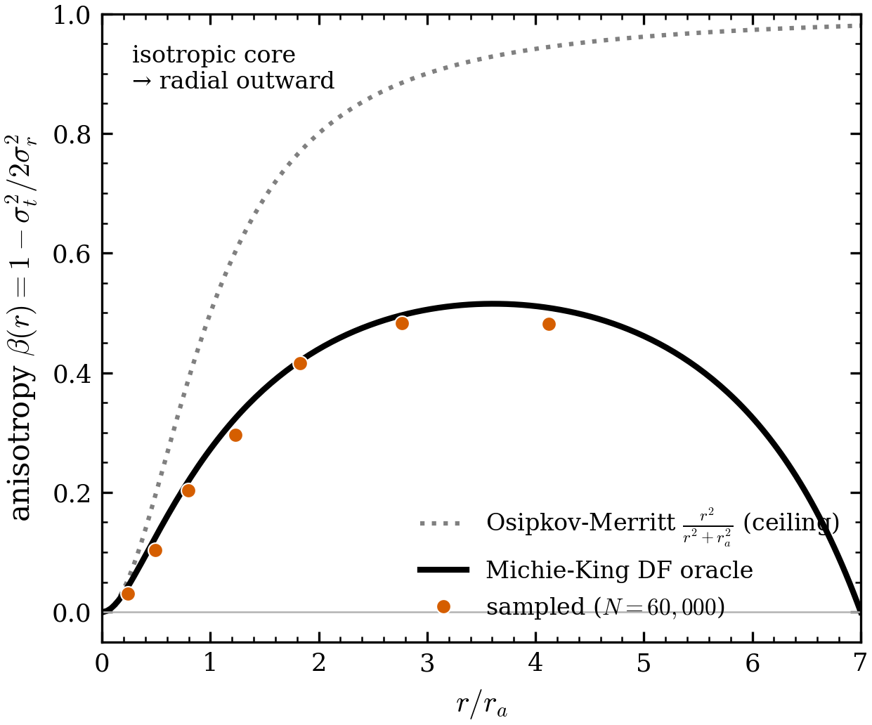
radially outward, and turns back toward isotropy at the tidal boundary. — Figure 1:**The anisotropy signature.** Sampled $\beta(r)=1-\sigma_t^2/2\sigma_r^2$ (points) tracks the **Michie-King DF oracle** (solid, the 2nd-moment integral of the exact DF) to max deviation 0.027 — and both sit **well below** the pure Osipkov-Merritt ceiling $r^2/(r^2+r_a^2)$ (dotted). $\beta\to0$ at the isotropic core, grows radially outward, and turns back toward isotropy at the tidal boundary.

Table-routed draws vs the exact (u_r,u_t) quadrature oracle (W_0=7,
r_a=8, N=2\times10^4). Since the 2026-06 memory batch,
MichieVelocityDF draws speeds from the anisotropic CDF table at g=1
(Michie ≡ LIMEPY g{=}1 anisotropic — change-of-variables proven and
brute-force verified), with the original 2-D quadrature retained as
speed_method="quadrature". (a) Speed distributions: KS D = 6.7\times10^{-3}
(gate <0.02; unpaired comparison — the two paths consume keys in different
orders). (b) Measured \beta(r): \max|\Delta\beta| = 0.042 (gate <0.06).
Script: scripts/validate_speed_routing.py; see
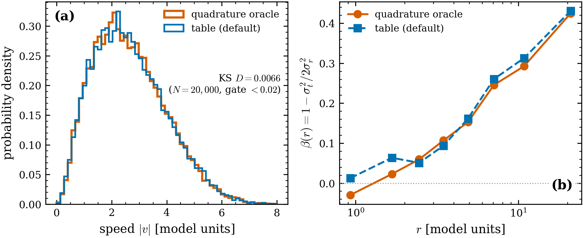
performance & memory. — Figure 2:**Table-routed draws vs the exact $(u_r,u_t)$ quadrature oracle ( $W_0=7$ , $r_a=8$ , $N=2\times10^4$ ).** Since the 2026-06 memory batch, `MichieVelocityDF` draws speeds from the anisotropic CDF table at $g=1$ (Michie ≡ LIMEPY $g{=}1$ anisotropic — change-of-variables proven and brute-force verified), with the original 2-D quadrature retained as `speed_method="quadrature"`. (a) Speed distributions: KS $D = 6.7\times10^{-3}$ (gate $<0.02$ ; unpaired comparison — the two paths consume keys in different orders). (b) Measured $\beta(r)$ : $\max|\Delta\beta| = 0.042$ (gate $<0.06$ ). Script: `scripts/validate_speed_routing.py`; see performance & memory.

Anisotropic dispersions and equilibrium. (a) The radial dispersion
\sigma_r exceeds the per-component tangential \sigma_t by a margin that widens
outward — the kinematic signature of radial anisotropy. (b) Every velocity is
bound, v\le v_{\rm esc}(r) — 100%. (c) The unscaled IC is virial,
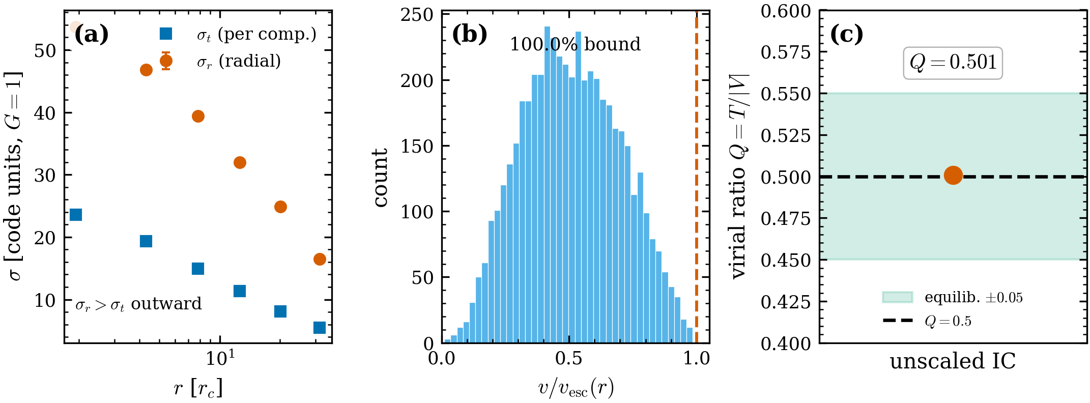
Q=0.501, with no external rescale (self-consistent \sigma^2=GM/9r_c\mu). — Figure 3:**Anisotropic dispersions and equilibrium.** (a) The radial dispersion $\sigma_r$ exceeds the per-component tangential $\sigma_t$ by a margin that widens outward — the kinematic signature of radial anisotropy. (b) Every velocity is bound, $v\le v_{\rm esc}(r)$ — **100%**. (c) The unscaled IC is virial, **$Q=0.501$** , with no external rescale (self-consistent $\sigma^2=GM/9r_c\mu$ ).

$Density and the King limit. As r_a\to\infty the Michie density coincides with the isotropic King profile (max rel 2.7\times10^{-3}); finite r_a (radial anisotropy) makes the model more extended (r_t/r_c=56 at r_a=8 vs 33.8 for King).$

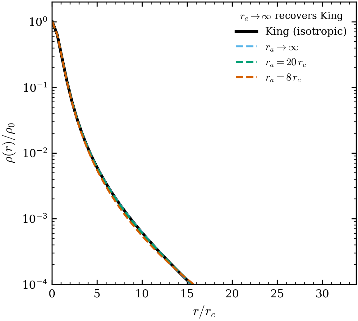
Figure 4:Density and the King limit. As $r_a\to\infty$ the Michie density coincides with the isotropic King profile (max rel $2.7\times10^{-3}$ ); finite $r_a$ (radial anisotropy) makes the model more extended ( $r_t/r_c=56$ at $r_a=8$ vs 33.8 for King).

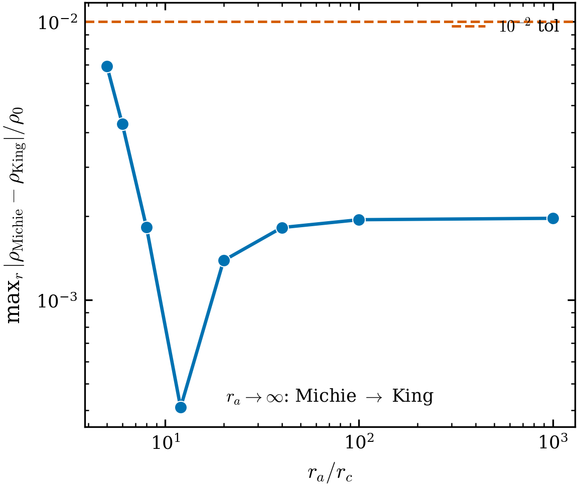
$Isotropic-limit convergence. The maximum density deviation from King falls with r_a/r_c, reaching \sim2\times10^{-3} (an ODE-grid floor) by r_a=10^3 — well inside the 10^{-2} tolerance. The dip near r_a\!\sim\!12 is a genuine density-profile crossing.$

Figure 5:Isotropic-limit convergence. The maximum density deviation from King falls with $r_a/r_c$ , reaching $\sim2\times10^{-3}$ (an ODE-grid floor) by $r_a=10^3$ — well inside the 10^-2 tolerance. The dip near $r_a\!\sim\!12$ is a genuine density-profile crossing.

Differentiability¶

The Michie structural parameters are differentiable through the diffrax ODE solve and the jax.lax.scan sampling, enabling gradient-based / HMC inference of the anisotropic model.

Gradient validation (autodiff vs central finite difference). \partial(\text{obs})/\partial\theta
for (a) W_0, (b) r_c, (c) M_{\rm tot}: autodiff and finite difference agree to
max rel err 1\times10^{-7}, 1\times10^{-8}, 7\times10^{-7}, so the anisotropic
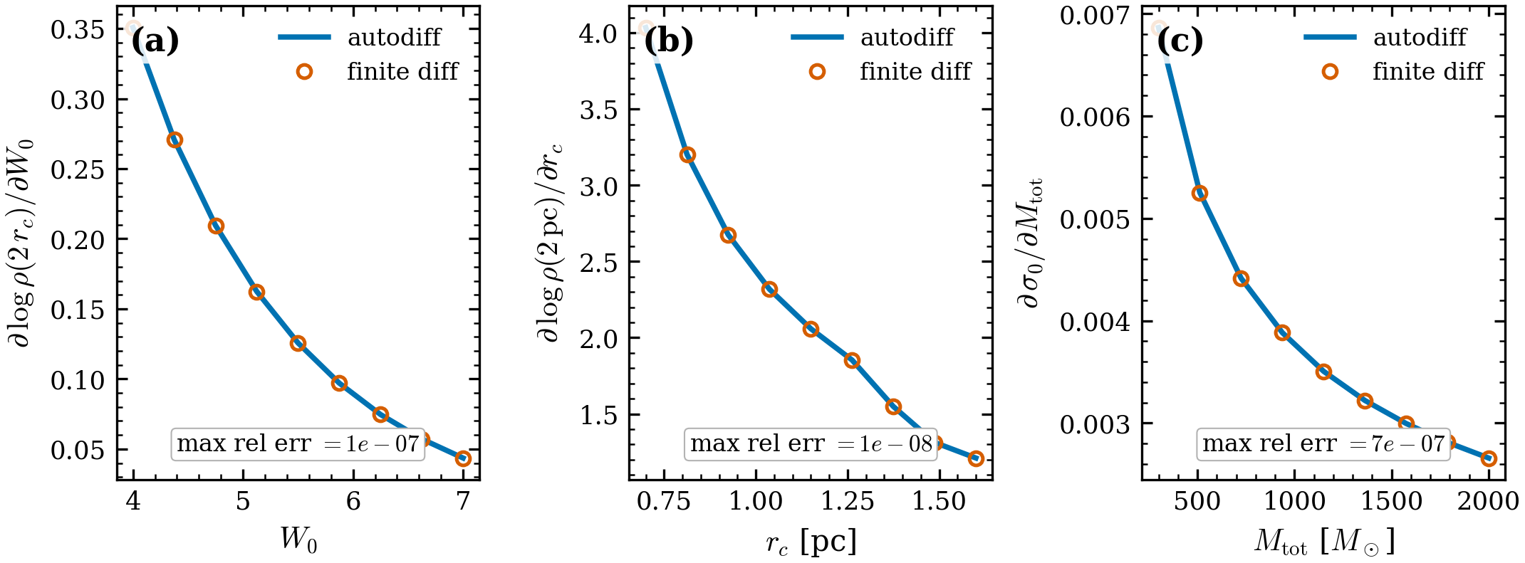
model can be fit jointly with the structural parameters. — Figure 6:**Gradient validation (autodiff vs central finite difference).** $\partial(\text{obs})/\partial\theta$ for (a) $W_0$ , (b) $r_c$ , (c) $M_{\rm tot}$ : autodiff and finite difference agree to max rel err $1\times10^{-7}$ , $1\times10^{-8}$ , $7\times10^{-7}$ , so the anisotropic model can be fit jointly with the structural parameters.

Equilibrium-dispersion

\partial\sigma/\partial W_0

for OED/Fisher (2026-06-17)

The OED/Fisher forward model differentiates the equilibrium dispersion jeans_dispersion / project_dispersion, which interpolate a master radial table back to the query radii. That back-interpolation was a piecewise-linear $C^0$ jnp.interp: as the truncation radius $r_t(W_0)$ moved the table’s grid nodes, the interpolant’s slope jumped at a fixed query radius and kinked $\partial\sigma/\partial W_0$ , so a coarse finite difference reported a $\sim 5\times10^{-3}$ inconsistency. The fix is a monotone $C^1$ (PCHIP) back-interpolation, which removes the slope jump: the Michie- $W_0$ dispersion gradient is now FD-consistent ( $5.1\times10^{-3}\to3.5\times10^{-4}$ at the gate step), model-general across King/Michie/EFF/Plummer. Caveat: beyond $W_0\approx7$ (at $r_a=5\,r_c$ ) the Michie model nears its mass-divergence ( $r_t\to\infty$ ); the gradient stays correct (a finite difference converges to autodiff as the step shrinks) but a fixed-step FD is a poor truth-proxy there, so the gradient gate runs in the well-truncated $W_0=6$ regime.

How to run¶

# physics tests (~22 s on CPU)
pytest tests/validation/test_michie_physics.py -q

# regenerate the five figures with PASS/FAIL tables
python scripts/validate_michie.py

What this suite does not test¶

Multi-mass anisotropic equilibrium — single-mass Michie-King is covered; the multi-mass generalization is part of the lowered-model-family roadmap.

References¶

Michie (1963) (anisotropy term) and King (1966) (lowered cutoff). The per-paper notes are in the bibliography; theory and the DF derivation at Michie-King anisotropic model.

References¶

Michie, R. W. (1963). On the distribution of high energy stars in spherical stellar systems. Monthly Notices of the Royal Astronomical Society, 125, 127–139. 10.1093/mnras/125.2.127
King, I. R. (1966). The structure of star clusters. III. Some simple dynamical models. The Astronomical Journal, 71, 64–75. 10.1086/109857