IMF statistics validation - progenax — differentiable initial conditions for N-body simulations

The released IMF samplers — piecewise power-law (Salpeter (1955), Kroupa (2001)), the Chabrier (2003) lognormal+power-law, and the Maschberger (2013) smooth bridging form — plus the internal TaperedPowerLaw and Schechter variants (used inside the package; not in the public progenax.__all__) — sampled by exact inverse-CDF (no rejection). Test file: tests/validation/test_imf_physics.py (see the test dashboard for the live per-suite count); figures: scripts/validate_imfs.py (5 figures, PASS/FAIL per panel, PNG + PDF). Theory at Classical IMFs (Salpeter, Kroupa, Chabrier, Maschberger).

Key result: the published slopes are recovered from samples, and the means are exact

Sampling 10⁵ stars and re-fitting the slope by maximum likelihood recovers every published $\alpha$ to within finite- $N$ error (Salpeter $2.347\pm0.004$ vs 2.35; the three Kroupa segments $0.294/1.297/2.301$ vs $0.3/1.3/2.3$ ). The differentiable mean_mass() matches a 200k-point log-grid reference to $\le1.2\times10^{-4}$ for all six IMFs — using the closed-form (power laws) or log-grid (smooth) integral precisely because a linear grid under-resolves the steep low-mass spike (shown below). Gradients of the inference-layer likelihood are exact (AD vs finite difference, rel err $\le10^{-5}$ ).

What is verified¶

Each row maps to assertions in test_imf_physics.py. Measured values are regenerated by scripts/validate_imfs.py ( $N=10^5$ samples, seed 42; KS at $N=2\times10^4$ ).

Property	Tolerance (as tested)	Measured	Anchor
Salpeter slope recovered (sample MLE)	$\|\Delta\alpha\| < 0.05$	$2.347\pm0.004$	Salpeter (1955) $\alpha=2.35$
Kroupa 3 segment slopes recovered	$\|\Delta\alpha\| \leq 0.08$	$0.294 / 1.297 / 2.301$	Kroupa (2001) $0.3/1.3/2.3$
Chabrier high-mass tail slope	$\|\Delta\alpha\| < 0.06$	$2.315\pm0.010$	Chabrier (2003) $\alpha=2.3$
Maschberger asymptotic slope	$\|\Delta\alpha\| < 0.15$	$2.358\pm0.158$	Maschberger (2013) $\alpha=2.3$
PDF coverage (hist vs analytic $m\,\xi$ )	median rel $< 0.05$	$0.018 / 0.020 / 0.019$	Chabrier / Kroupa / Maschberger
CDF goodness-of-fit (KS)	$D < D_{\rm crit}=0.0096$	$0.0049 / 0.0072 / 0.0082$	Salpeter / Maschberger / Chabrier
KS $p$ -value	$p > 0.01$	$0.71 / 0.26 / 0.13$	consistent with exact sampling
`mean_mass()` vs 200k log-grid ref	rel $< 10^{-2}$ (6 IMFs)	$\leq 1.2\times10^{-4}$	independent reference integral
Linear-grid failure mode (adversarial)	log grid $\ll$ linear grid	$1.2\times10^{-6}$ vs $1.3\times10^{-2}$	steep $m^{-2.35}$ low-mass spike
Inference-layer gradient (AD vs FD)	rel err $< 10^{-3}$	$\leq 1\times10^{-5}$	`IMFParams` $\partial\,$ NLL $/\partial\alpha$
Truncated power-law clipping	all samples in $[m_{\min}, m_{\max}]$	no rejection (inverse CDF)	`TruncatedIMF` renormalization

Provenance

The implemented constants were checked against the four primary papers directly (per-paper notes: Salpeter (1955), Kroupa (2001), Chabrier (2003), Maschberger (2013)): Salpeter $\alpha=2.35$ (Eq. 5, the logarithmic MF $\Rightarrow$ $dN/dm$ slope 2.35); Kroupa breaks $0.08/0.5$ and slopes $0.3/1.3/2.3$ (Eq. 2); Chabrier single-star disk $m_c=0.079$ , $\sigma=0.69$ , high-mass $x=1.3 \Rightarrow \alpha=2.3$ (Table 2, with the $1/(m\ln 10)$ Jacobian to $dN/dm$ ); Maschberger $\mu=0.2$ , $\alpha=2.3$ , $\beta=1.4$ and the closed-form quantile (Table 1). The recovered-slope figure below is therefore both a sampler check and a confirmation of those PDF-verified constants. See the per-paper notes in the bibliography.

Figures¶

Generated by scripts/validate_imfs.py (PASS/FAIL per panel; PNG + PDF vector).

Recovered slopes (headline). Sampling 10^5 stars and re-fitting the slope by
bounded-power-law maximum likelihood recovers every published \alpha along the
y=x line: Salpeter 2.35, the three Kroupa segments 0.3/1.3/2.3, the Chabrier
high-mass tail 2.3, and the Maschberger asymptotic 2.3. Error bars are bootstrap
standard errors — wide for Maschberger because only \sim120 stars exceed
20\,M_\odot in the window. The four near-coincident points at the top right all sit
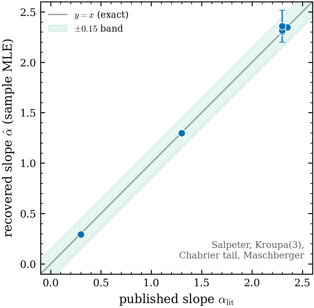
at \alpha\simeq2.3–2.35. — Figure 1:**Recovered slopes (headline).** Sampling 10⁵ stars and re-fitting the slope by bounded-power-law maximum likelihood recovers every published $\alpha$ along the $y=x$ line: Salpeter 2.35, the three Kroupa segments $0.3/1.3/2.3$ , the Chabrier high-mass tail 2.3, and the Maschberger asymptotic 2.3. Error bars are bootstrap standard errors — wide for Maschberger because only $\sim120$ stars exceed $20\,M_\odot$ in the window. The four near-coincident points at the top right all sit at $\alpha\simeq2.3$ –2.35.

PDF shape coverage. Sampled histograms (points) overlay the analytic
m\,\xi(m) (solid) across the full mass range for (a) the Chabrier
lognormal+power-law, (b) the Kroupa piecewise power law, and (c) the Maschberger
smooth bridging form — median relative deviation \leq2\% in every case. The
lognormal turnover, the segment breaks at 0.08 and 0.5\,M_\odot, and the smooth
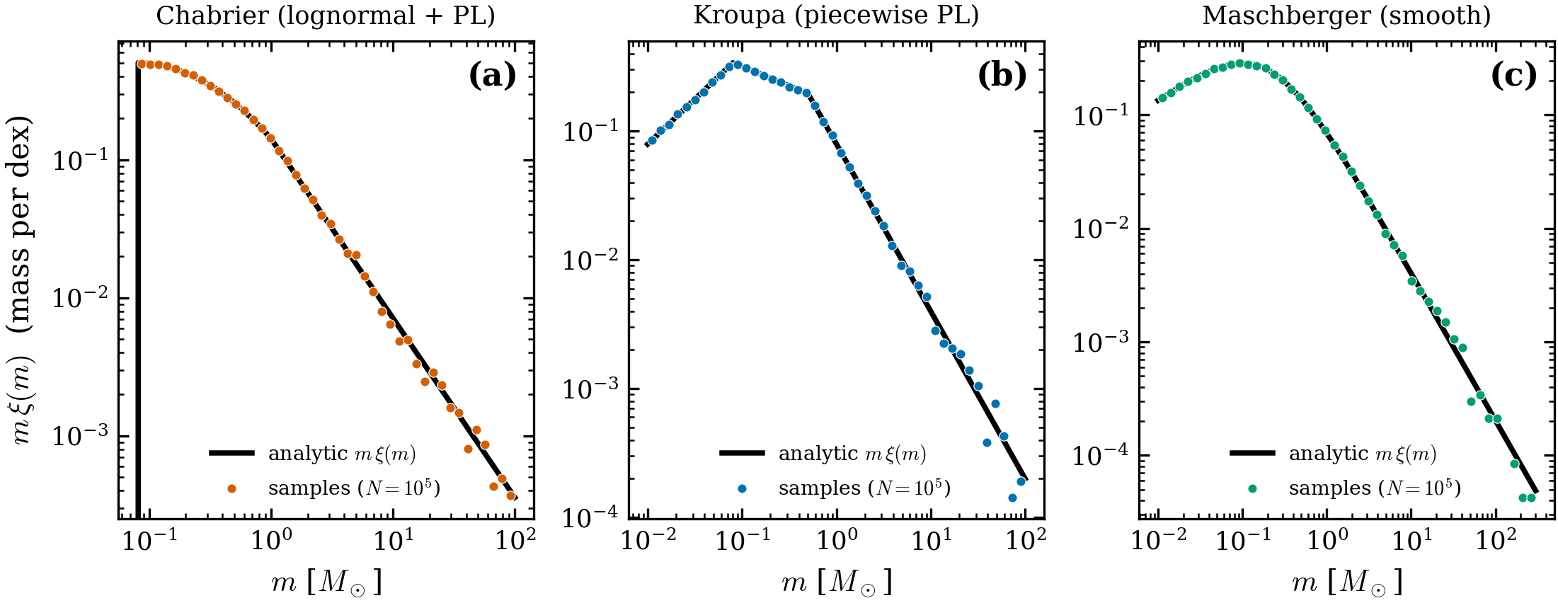
peak are all reproduced. — Figure 2:**PDF shape coverage.** Sampled histograms (points) overlay the analytic $m\,\xi(m)$ (solid) across the full mass range for (a) the Chabrier lognormal+power-law, (b) the Kroupa piecewise power law, and (c) the Maschberger smooth bridging form — median relative deviation $\leq2\%$ in every case. The lognormal turnover, the segment breaks at 0.08 and $0.5\,M_\odot$ , and the smooth peak are all reproduced.

CDF coverage and the KS test. Empirical CDFs (points) lie on the analytic
F(m) (solid) for both the analytic-PPF samplers (Salpeter, Maschberger) and the
Newton-PPF sampler (Chabrier). The Kolmogorov–Smirnov statistic is below the 0.05
critical value D_{\rm crit}=0.0096 in all three cases (p=0.71/0.26/0.13) — the
samples are statistically consistent with the exact distributions, including the
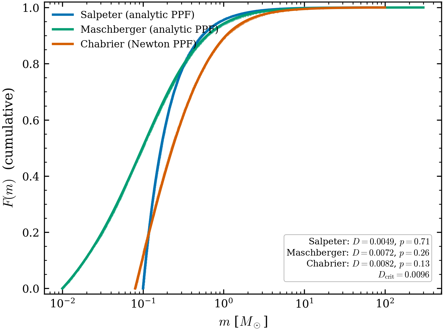
iterative Chabrier inverse. — Figure 3:**CDF coverage and the KS test.** Empirical CDFs (points) lie on the analytic $F(m)$ (solid) for both the analytic-PPF samplers (Salpeter, Maschberger) and the Newton-PPF sampler (Chabrier). The Kolmogorov–Smirnov statistic is below the 0.05 critical value $D_{\rm crit}=0.0096$ in all three cases ( $p=0.71/0.26/0.13$ ) — the samples are statistically consistent with the exact distributions, including the iterative Chabrier inverse.

Mean-mass accuracy and the linear-grid failure mode (adversarial). (a) The
differentiable mean_mass() matches a 200k-point log-grid reference to
\leq1.2\times10^{-4} for all six IMFs — exact (\sim10^{-10}) for the closed-form
power laws. (b) Why the log grid matters: estimating \langle m\rangle for the steep
Salpeter spike on a linear grid stalls at \sim1\% error even at N=4000
points, while the log grid converges to 10^{-6}. This is the documented reason the
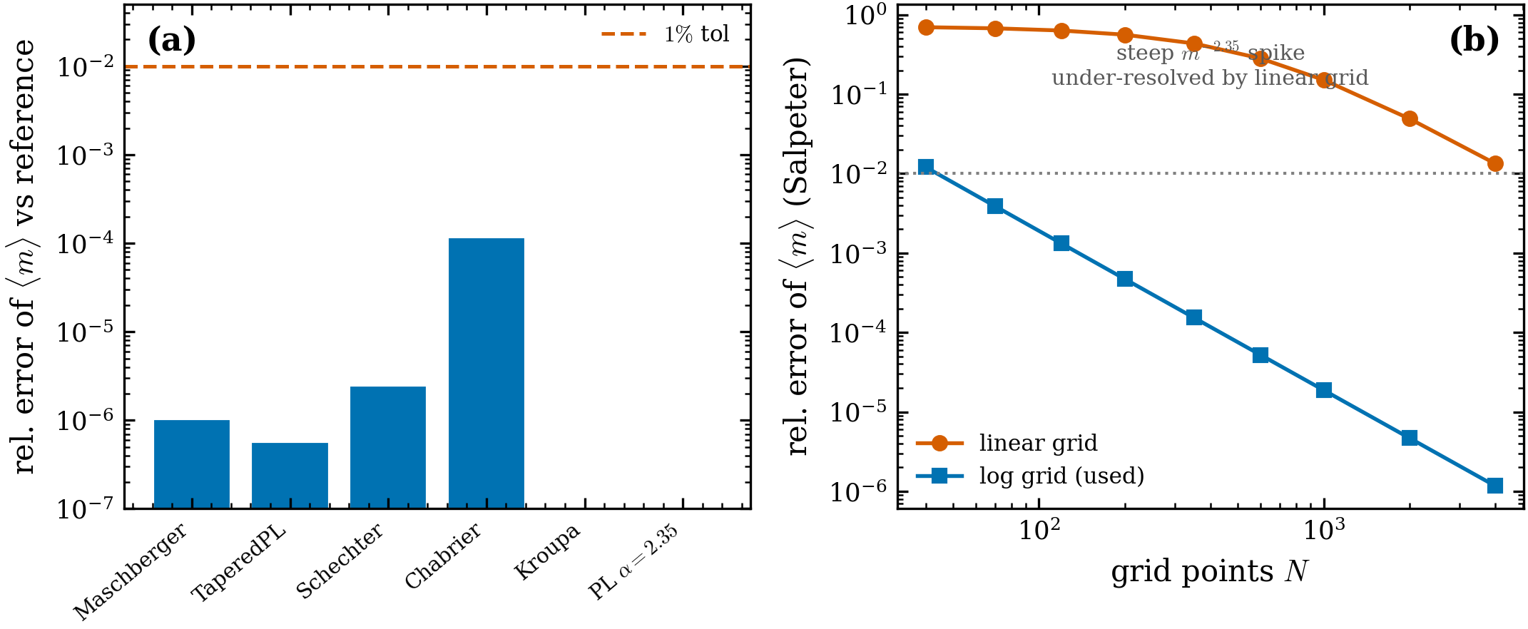
implementation never uses a linear-grid trapezoid. — Figure 4:**Mean-mass accuracy and the linear-grid failure mode (adversarial).** (a) The differentiable `mean_mass()` matches a 200k-point log-grid reference to $\leq1.2\times10^{-4}$ for all six IMFs — exact ( $\sim10^{-10}$ ) for the closed-form power laws. (b) Why the log grid matters: estimating $\langle m\rangle$ for the steep Salpeter spike on a **linear** grid stalls at $\sim1\%$ error even at $N=4000$ points, while the log grid converges to 10^-6. This is the documented reason the implementation never uses a linear-grid trapezoid.

Inference-layer gradient validation. For the differentiable IMFParams
likelihood, autodiff (line) and central finite difference (circles) of
\partial\,NLL/\partial\alpha agree to max rel err \leq10^{-5} for (a) the
high-mass slope \alpha_3 and (b) \alpha_2. The gradient’s zero crossing (star)
is the maximum-likelihood slope, recovering the input (2.32, 2.31 vs the
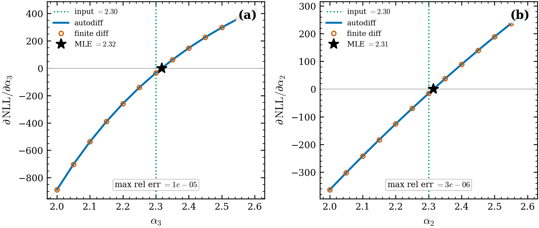
generating 2.30) — so the IMF can be fit by gradient descent / HMC. — Figure 5:**Inference-layer gradient validation.** For the differentiable `IMFParams` likelihood, autodiff (line) and central finite difference (circles) of $\partial\,$ NLL $/\partial\alpha$ agree to max rel err $\leq10^{-5}$ for (a) the high-mass slope $\alpha_3$ and (b) $\alpha_2$ . The gradient’s zero crossing (star) is the maximum-likelihood slope, recovering the input (2.32, 2.31 vs the generating 2.30) — so the IMF can be fit by gradient descent / HMC.

Differentiability¶

All IMF sampling uses exact inverse-CDF with a fixed iteration count (analytic for the power laws and Maschberger; a 30-step Newton solve for Chabrier), so gradients flow through both the samples (reparameterization) and the structural parameters. The progenax.imf.differentiable layer (log_prob_masses, sample_masses_from_params, individual_mass_nll over IMFParams) is the gradient-based inference target validated in Figure 5.

How to run¶

# physics tests (~8 s on CPU)
pytest tests/validation/test_imf_physics.py -q

# regenerate the five figures with PASS/FAIL tables
python scripts/validate_imfs.py

What this suite does not test¶

Binary contamination bias — the forward model + binary-aware likelihood are covered separately at Binary-aware IMF validation.
Environment dependence — the IGIMF / BirthEnvironment mapping is documented at Environment-dependent IMFs but is not part of this validation suite.

References¶

Salpeter (1955), Kroupa (2001), Chabrier (2003), Maschberger (2013). Per-paper notes in the bibliography; theory at Classical IMFs (Salpeter, Kroupa, Chabrier, Maschberger).

References¶

Salpeter, E. E. (1955). The luminosity function and stellar evolution. The Astrophysical Journal, 121, 161–167. 10.1086/145971
Kroupa, P. (2001). On the variation of the initial mass function. Monthly Notices of the Royal Astronomical Society, 322, 231–246. 10.1046/j.1365-8711.2001.04022.x
Chabrier, G. (2003). Galactic stellar and substellar initial mass function. Publications of the Astronomical Society of the Pacific, 115, 763–795. 10.1086/376392
Maschberger, T. (2013). On the function describing the stellar initial mass function. Monthly Notices of the Royal Astronomical Society, 429, 1725–1733. 10.1093/mnras/sts479