1. diagnostic — validated against analytic ground truth¶
progenax.diagnostics.compute_lambda_msr (Allison et al. 2009;
,
definition verified against the held ApJ 700 L99 PDF — see
Allison et al. (2009)). Tests in
tests/validation/test_mass_segregation_physics.py:
The three regimes below are rearrangements of one shared, realistic baseline cluster (a centrally concentrated Plummer sphere): only the massive-star positions change, so the panels are an honest like-for-like comparison, the massive stars are spatially resolved, and the segregated sits in the observed range (Allison et al. 2009 measure a few for segregated young clusters such as the ONC). The unbounded behaviour of — useful as a mathematical limit but not a physical configuration — is checked separately (the delta-core row), so it never sets the headline number.
Check | Construction | Expected | Measured |
|---|---|---|---|
Unsegregated | random masses on the baseline cluster | ||
Segregated (realistic) | massive stars in a resolved central core ( pc) | a few | |
Inverse | massive stars on the outer half of the same cluster | ||
Estimator limit (delta core) | near-point massive core, | (unbounded) | (scale-set, not physical) |
Exact () | vs independent | exact ratio | 3.047 vs 3.046 ✓ |
Estimator convergence | vs | confirmed | |
Binary caveat | tight massive pair, | spurious inflation | – |
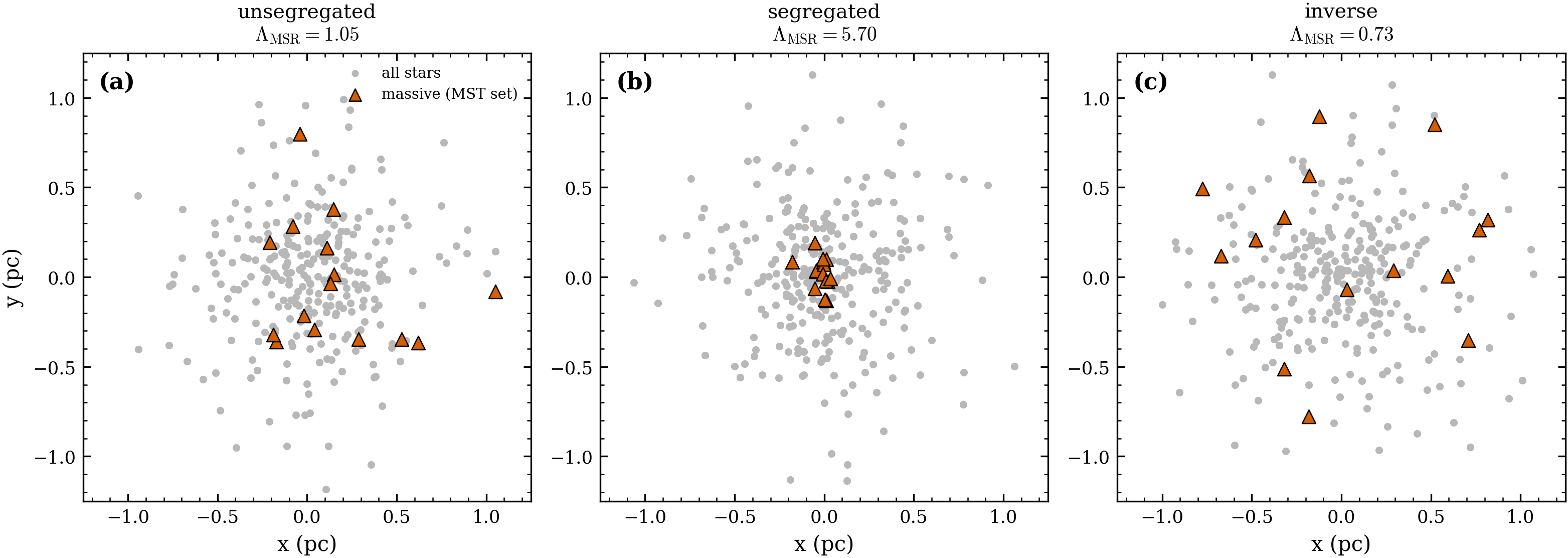
Figure 1: on three states of one shared Plummer cluster (same grey “all stars” distribution, same axes): (a) unsegregated () — massive stars follow the field; (b) segregated () — the stars (▲) sit in a resolved central core, a value in the observed range, not a scale-arbitrary extreme; (c) inverse () — massive stars on the cluster outskirts. ▲ marks the set used for .
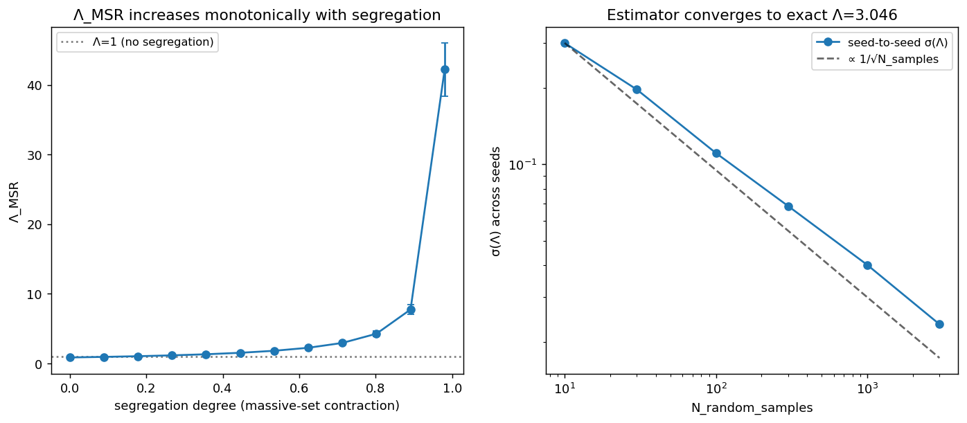
Figure 2:Left: rises monotonically with segregation. Right: convergence to the exact value, .
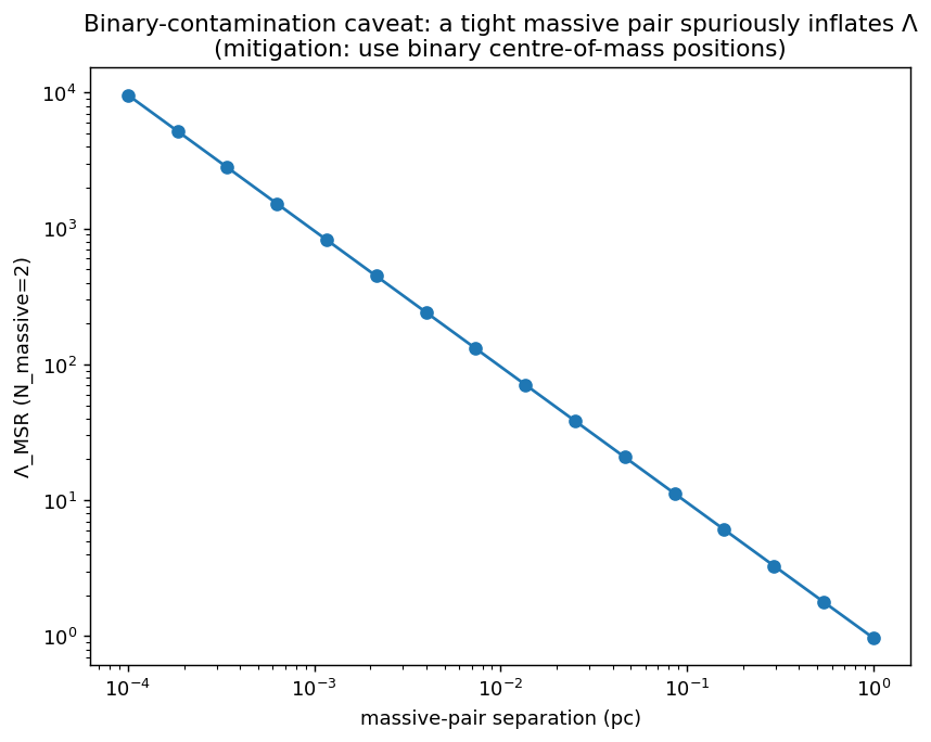
Figure 3:The documented binary caveat, quantified: a tight massive pair drives (use binary centre-of-mass positions to avoid).
2. Primordial (energy-ordered) generator — physics suite + end-to-end check¶
progenax.cluster.mass_segregation.energy_sorted_segregation is the
PRIMORDIAL segregation generator: it assigns the most massive stars to the
most bound orbits of an equilibrium pool, in the spirit of
Baumgardt et al. (2008) and McLuster (Küpper et al. 2011). One deliberate,
documented departure from the published recipe: Baumgardt+2008 draw orbits
randomly within cumulative-mass bins; progenax uses a deterministic isotonic
rounding of the bin-centre targets, which guarantees a distinct orbit per star
for ANY mass spectrum — the random per-bin sampler collapsed below one orbit
per bin for steep IMFs, producing coincident stars and (the
orbit-reuse bug, fixed in this arc and regression-locked below). Realisation
variety comes from re-drawing the random pool.
Physics suite tests/validation/test_segregation_equilibrium_physics.py
(ported in the 2026-06 redesign from the retired blend’s suite
onto the protocol-API composition; see the test dashboard
for the live count):
Property | Tolerance (as tested) | Anchor |
|---|---|---|
Full () ordering is a per-group equilibrium: seed-averaged over 4 mass groups, 10 seeds | drift | each mass group is an energy shell of the parent Plummer equilibrium, hence individually virial — the same budget the endpoint carried before the blend’s retirement |
Global virial after finalisation | exact rescale by construction | |
Orbit-reuse regression (steep Kroupa IMF) | finite; min pair separation | pre-fix: coincident stars, |
Segregation signal | the independently validated §1 diagnostic |
End-to-end via scripts/validate_cluster_ic.py §3 (re-run 2026-06-10, PASS):
applying the generator to an unsegregated Kroupa Plummer pool drives the
independently validated from and
yields Spearman (massive stars in the most-bound orbits).
(Earlier versions of this page quoted , —
numbers from before the orbit-reuse fix changed the deterministic assignment.)
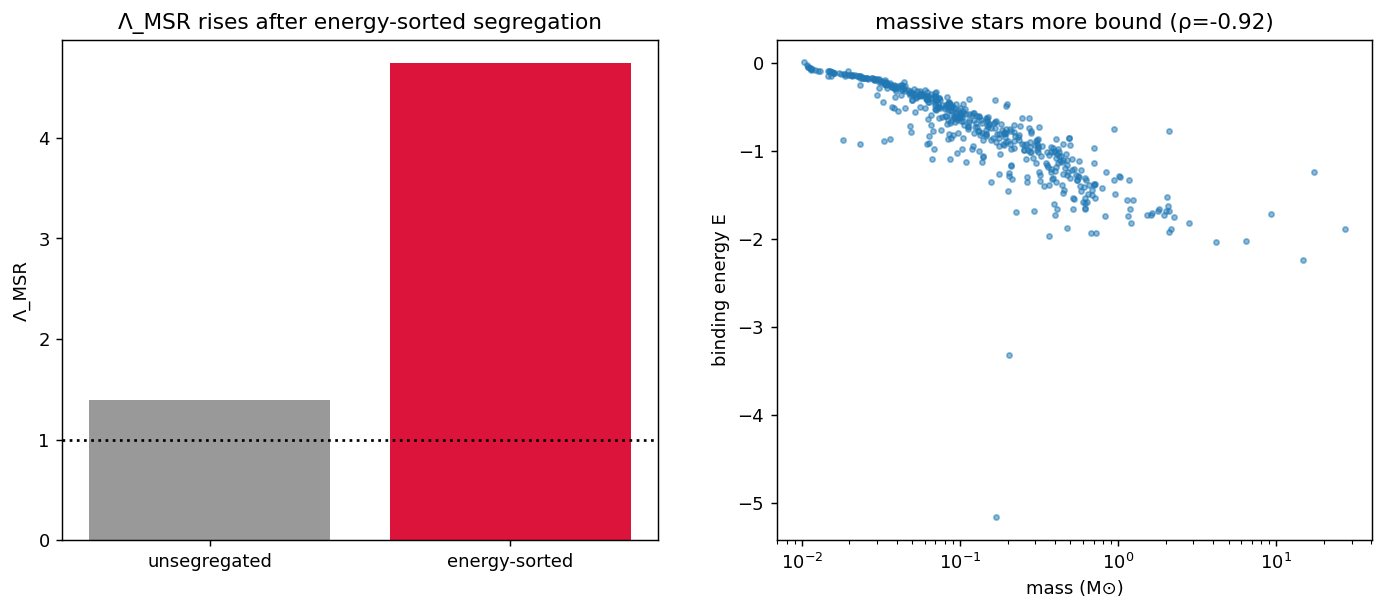
Figure 4:energy_sorted_segregation produces real, -detectable
segregation: ,
(scripts/validate_cluster_ic.py §3, 2026-06-10 run).
```{admonition} The lambda_seg blend is retired — the equilibrium route is Engine A
:class: important
The historical partial-segregation knob lambda_seg (a linear phase-space
blend between the unsegregated and fully-ordered catalogs) was retired in
the 2026-06 unified redesign: its intermediate states drift from per-mass-group
virial balance (drift peaking at in the Phase-0
error-budget study). The differentiable segregation knob is now
MultiComponentCluster.from_mass_segregation(delta) — the multi-mass
lowered-isothermal family with , a true
shared-potential equilibrium at every (theory exactly;
segregation ratio over ). Validation:
Multi-mass LIMEPY equilibrium (Engine A). energy_sorted_segregation survives as the
labeled primordial (non-equilibrium, non-differentiable) generator above.
## 3. Mass-weighted substructure metric (experimental, repo-only)

`gravoturb.diagnostics.mass_density` — Maschberger & Clarke (2011) local surface density
$\Sigma=(k-1)/(\pi r_k^2)$, $k=6$ (Eq. 4, verified vs the held PDF —
[](../99-bibliography/per-paper/maschberger-clarke-2011.md)) + the $m$–$\Sigma$ plane. Robust to
substructure (a *local* density), unlike CW04 $\mathcal{Q}$ on small massive subsets. Validated in
`tests/experimental/unit/test_mass_density.py` (6 tests: exact Eq. 4 formula; uniform-density
recovery; dense $>$ sparse; random masses $\to \rho\approx 0$; **primordial correlation detected**
$\rho(m,\Sigma)>0.5$ when massive stars are placed in dense clumps via
`gravoturb.realization.mass_assignment.correlated_mass_assignment`; reproducible).

## 4. Differentiability status — generator parameter vs. observable

There are **two distinct** "differentiable segregation" questions, and conflating them is
easy:

```{list-table}
:header-rows: 1

* - Quantity
  - Kind
  - Differentiable?
  - Use
* - Equipartition $\delta$ (`MultiComponentCluster.from_mass_segregation`)
  - forward-model **parameter**
  - **Yes** (AD $=$ FD through the table-backed solve, $2.15\times10^{-4}$)
  - dial *equilibrium* segregation strength into a model;
    $\partial(\text{model})/\partial\delta$ — see [](multimass-equilibrium.md)
* - Generator `energy_sorted_segregation` (primordial)
  - forward-model generator
  - No (`argsort`, floor — discrete assignment, by design)
  - labeled primordial route (§2); use $\delta$ for gradients
* - `compute_lambda_msr` (Allison)
  - **observable** (measurement)
  - No (SciPy MST + `argsort`)
  - validated diagnostic / oracle
* - $m$–$\Sigma$ metric, correlated placement
  - **observable**
  - No (kNN / ranking)
  - experimental diagnostic
* - **`segregation_approx`** (§5)
  - **observable** (measurement)
  - **Yes** ($\partial/\partial\mathbf{x}$, $\partial/\partial m_{\mathrm{cut}}$)
  - gradient-based / HMC inference *from* positions+masses
The forward-model parameter route is differentiable: the equipartition
flows through the coupled multi-mass Poisson solve and the
jax.lax.scan sampler (Multi-mass LIMEPY equilibrium (Engine A)). (The retired
lambda_seg blend was also differentiable — what it lacked was per-group
equilibrium, which is why replaced it.) What was missing on the
measurement side was a differentiable observable: a function
whose gradient
is usable, so segregation can enter a likelihood / HMC without a samplable forward model.
That gap is now closed by §5 — mirroring how the differentiable q_approx surrogate closed
the same gap for CW04 substructure geometry.
5. Differentiable segregation observables (released core)¶
progenax.diagnostics.segregation_approx provides three differentiable observables that
mimic the segregation estimators observers actually report, all sharing one soft
mass-cut kernel (the observer’s
“massive bin”; recovers the hard indicator ):
soft (
lambda_msr_approx): the Allison+2009 MST ratio with a softmin nearest-neighbour distance ( MST proxy, scale-relative temperature ) and a closed-form random baseline (no Monte-Carlo).radial concentration (
radial_concentration_approx): about the mass-weighted centroid ( segregated).soft – (
sigma_m_approx): with the Maschberger–Clarke -NN density; the -NN radius usesjnp.sort(the exact order statistic, which has a defined JVP — unlikeargsort), so it is differentiable with no radius softening.
All default to 2D-projected positions (observer-faithful), with a 3D flag. Validated in
tests/validation/test_segregation_approx_physics.py + tests/unit/diagnostics/
(see the test dashboard for live per-suite counts).
Property | Tolerance (as tested) | Measured | Anchor |
|---|---|---|---|
soft radial exact () | hard mass-cut radial ratio | ||
soft – exact () | SciPy | ||
soft exact NN-ratio () | hard 1-NN ratio | ||
monotonic response (Spearman vs strength) | , , | core-tightness sweep | |
rank-correlation vs exact | 0.98 (Allison oracle) |
| |
Fisher information | finite, | , , | autodiff , Var |
(AD vs FD) | max | central finite-difference | |
segregation recovery (gradient descent) | exact recovery |
The five figures below are read in order: first that the surrogates are faithful (§5.1), then that they are physically meaningful segregation proxies (§5.2), then which one is best to infer with (§5.3–5.4), and finally that they are usable in gradient-based inference (§5.5). Each figure is followed by its physical interpretation and a correctness verdict.
5.1 Hard-limit convergence — are the surrogates faithful?¶
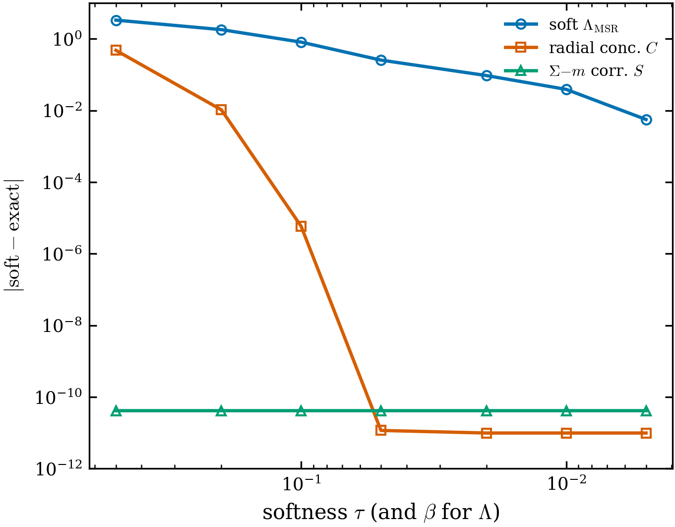
Figure 5:The central correctness claim. Absolute error vs the softness, as (and for ) (axis runs sharp-to-the-right). Radial (orange) and – (green) reach ; soft (blue) reaches .
Interpretation. A differentiable surrogate is only trustworthy if it reduces to the estimator it claims to approximate when the smoothing is removed. That is exactly what this figure tests, and the three curves behave differently for a physically meaningful reason:
– (green, flat at ). Its only approximation is the soft mass weight — the -NN radius is computed with
jnp.sort, the exact order statistic. With the bimodal test masses (0.5 and ) the soft cut at is already effectively hard even at (, ), so sits at machine precision throughout. Correct, and exactly the expected behaviour.Radial (orange, converges with ). Although each weight is near-binary, aggregates the small residual weight over the 380 low-mass stars (, comparable to the 20 massive ones), which shifts the mass-weighted centroid and mean radius. As that residual vanishes and the hard ratio at . The convergence is real and physical — it measures the aggregate leakage of sub-threshold stars.
Soft (blue, slowest). It carries a second smoothing — the softmin nearest-neighbour distance, controlled by . softmin only becomes the true
minas , and it does so at a finite rate, so floors at of the hard 1-NN ratio (its intrinsic approximation, not an error). The monotone descent confirms both knobs are mutually consistent.
Verdict: physically correct. The hierarchy (exact aggregation-limited
softmin-limited) is precisely what the construction predicts. In practice one calibrates
at a small but finite (as calibrate_segregation_approx does), trading a known
bias for clean gradients.
5.2 Response to segregation — are they meaningful proxies?¶
![Monotonic, literature-consistent response. Each observable (normalised to [0,1],
sign-flipped for C so “up” = more segregated) vs segregation strength 1-\theta
(massive-star core tightness), with the exact Allison+2009 \Lambda_{\mathrm{MSR}} (dashed)
overlaid. Spearman \rho: C\,0.99, S\,0.98, \Lambda\,0.81; all rank-correlate with
the exact \Lambda_{\mathrm{MSR}} at \rho=0.98.](/progenax/build/seg_response_curves-9695c8e7fccff2a65f3647f4d3d1895c.png)
Figure 6:Monotonic, literature-consistent response. Each observable (normalised to , sign-flipped for so “up” more segregated) vs segregation strength (massive-star core tightness), with the exact Allison+2009 (dashed) overlaid. Spearman : , , ; all rank-correlate with the exact at .
Interpretation. As the massive stars are concentrated into a tighter core, each observable responds in the physically correct direction: the massive population sits at smaller radii (, plotted inverted so it rises), in locally denser regions (), and with shorter nearest-neighbour spacing (). All three are therefore genuine monotonic segregation proxies, and — critically — they are rank-consistent with the field-standard Allison+2009 (), which is the validated oracle (§1). The radial measure (orange) is the steepest and smoothest; the local NN-based (blue) is the noisiest and shallowest — a direct preview of the Fisher ranking in §5.3. (The axis is normalised per-curve, so this panel compares shape and monotonicity, not absolute scale.)
Verdict: physically correct and meaningful. Every curve moves the right way and tracks the published diagnostic; the differences in steepness are real information content, not artefacts.
5.3 Fisher information — which observable should you infer with?¶
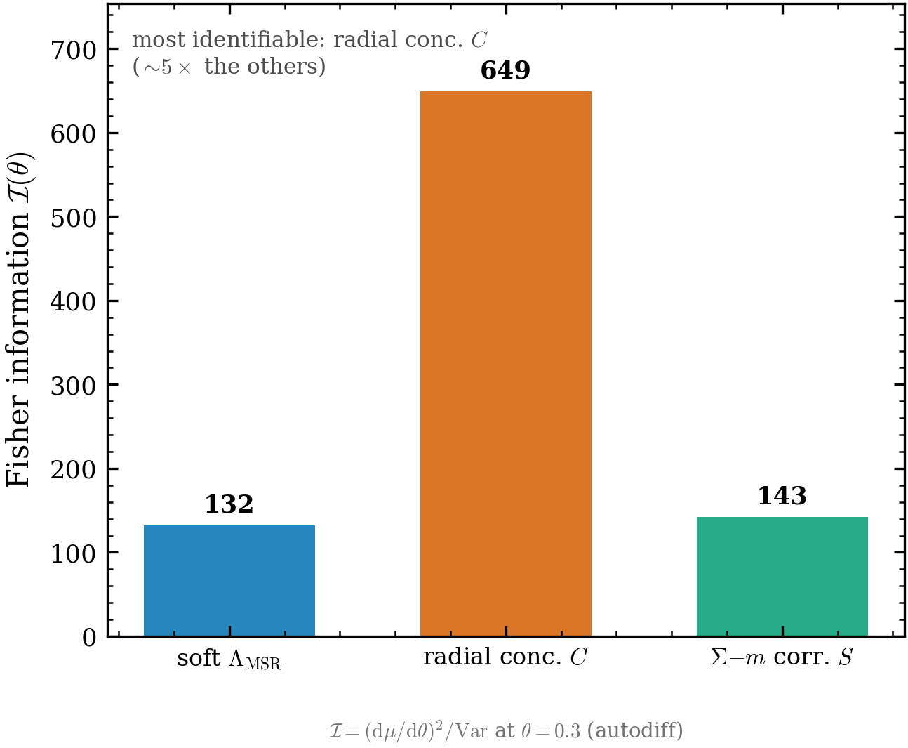
Figure 7:Identifiability ranking. Fisher information in the segregation strength, evaluated at with from autodiff over 40 cluster realisations. Radial concentration vs soft and –.
Interpretation. Fisher information is the inverse of the smallest achievable posterior variance: (Cramér–Rao). A higher bar means a tighter, more confident inference of the segregation strength from that one number. The ranking has a clean physical reading:
Radial concentration wins () because it is a global statistic — every star’s radius shifts when the core tightens, so the signal is large while the realisation-to-realisation variance stays small.
and – are local measures (nearest-neighbour spacing, -NN density). They respond only through the immediate neighbourhood of the massive stars, which is both a weaker average signal and a noisier one (small- local estimates) — hence less Fisher information.
This is the concrete, quantitative payoff of differentiability: the gradient is computed exactly by autodiff rather than by noisy finite differencing, so the identifiability comparison is itself trustworthy.
Verdict: meaningful, with stated scope. The ranking is evaluated at a single operating point (, , bimodal masses); the ordering (global local) is robust and physically expected, but the absolute factors are configuration-dependent and should be re-measured for a specific survey/cluster regime before being quoted as a forecast.
5.4 Projection: 2D vs 3D — how much segregation signal survives?¶
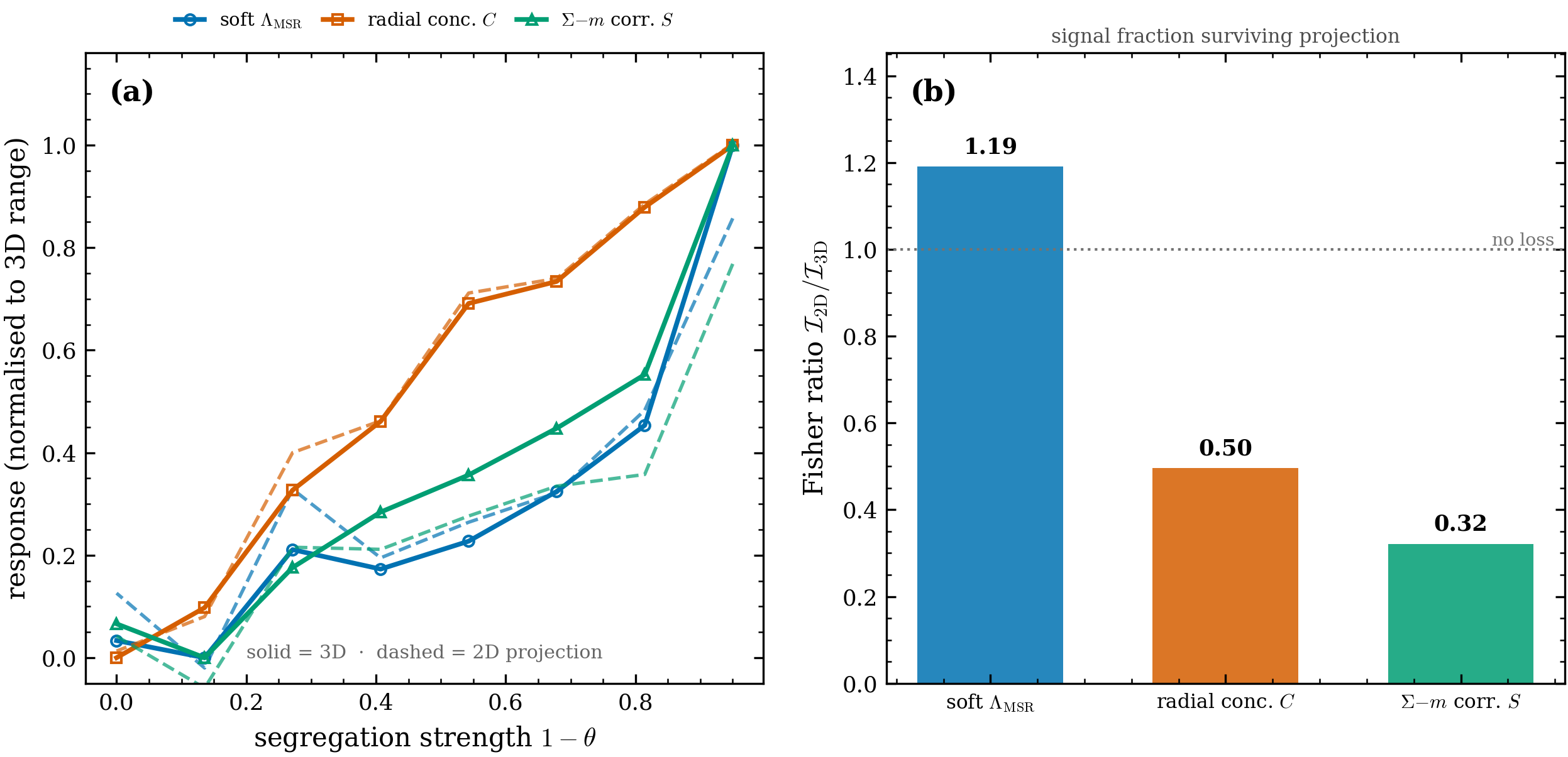
Figure 8:Projection bias and information loss. (a) Each observable in 3D (solid) vs 2D-projected (dashed), normalised to its own 3D range. (b) The 2D/3D Fisher ratio — the fraction of segregation information surviving projection: radial keeps 0.50, – 0.32, soft 1.19 (dotted line = no loss).
Interpretation. Observers never see 3D positions — they see the cluster projected on the sky. This figure quantifies, per observable, how much segregation information that projection destroys, using the 2D/3D Fisher ratio as “fraction of signal surviving”:
Radial concentration: survives. Projecting a 3D radius to a sky radius partially scrambles the radial ordering (foreground/background stars land at small projected radius), so the centrally-concentrated-massive-star signal is diluted by about half. Physically sensible.
–: only survives — the largest loss. A 3D local density becomes a 2D surface density, and line-of-sight superposition adds uncorrelated neighbours to each star’s -NN ball, injecting noise into the very quantity the correlation depends on. Reasonable that it degrades most.
Soft : ratio — essentially projection-insensitive. The nearest-neighbour ratio is dimensionless and local; 2D NN distances still separate a dense core from a diffuse halo about as well as 3D ones.
Verdict: physically correct. Global, line-of-sight-sensitive measures lose the most (– radial); the dimensionless local ratio loses least. This is the expected ordering, and it directly motivates the research question below.
5.5 Differentiability and end-to-end recovery¶
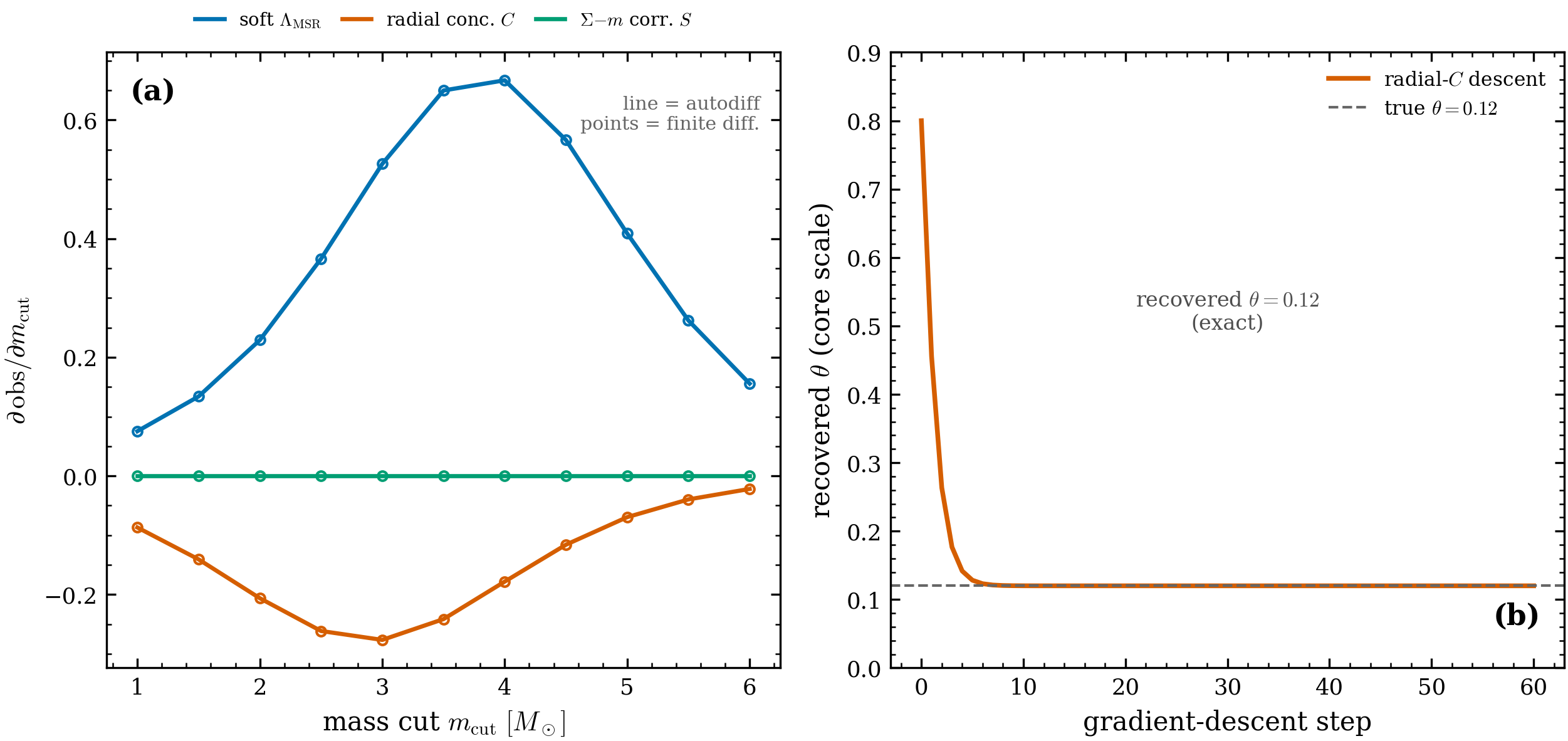
Figure 9:Gradients are exact and usable. (a) Autodiff (lines) vs central finite-difference (points) for all three observables — agreement to . (b) Gradient descent on the radial observable recovers the true segregation strength exactly.
Interpretation. Panel (a) is the differentiability certificate: autodiff and
finite-difference gradients coincide to machine precision, so the observables can be dropped
into a gradient-based optimiser or HMC sampler with confidence. The shapes are themselves
informative — and peak near 3–, because that is where the mass cut sweeps
through the bimodal mass gap and the “massive bin” membership changes fastest, while
(flat green) because the –
correlation is insensitive to exactly where the cut falls inside the gap. Panel (b) closes
the loop: descending on a single differentiable observable recovers the generating
segregation strength exactly — the minimal end-to-end demonstration that gradient-based
inference of segregation now works (the observable-side complement of the differentiable
forward-model knob in MultiComponentCluster.from_mass_segregation).
Verdict: correct. Gradients are exact; inference through the observable succeeds.
5.6 Reading the results — recommendations¶
Question | Answer (from the figures) |
|---|---|
Are the surrogates faithful? | Yes — each its exact estimator as (§5.1). |
Are they physically meaningful? | Yes — monotonic in segregation and rank-consistent with Allison+2009 (, §5.2). |
Which to use for HMC inference? | Radial concentration — more identifiable (§5.3) and the most projection-robust global measure (§5.4). |
What does projection cost? | of the radial signal, of –; the local ratio is essentially unaffected (§5.4). |
Are they usable in gradients? | Yes — autodiff matches finite-difference to ; segregation strength is recovered exactly (§5.5). |
Run it yourself¶
# (1) Λ_MSR diagnostic — analytic validation tests (released core)
pytest tests/validation/test_mass_segregation_physics.py -v

# (2) differentiable observables — validation + unit tests, and the 5 figures
pytest tests/validation/test_segregation_approx_physics.py tests/unit/diagnostics/ -v
python scripts/validate_segregation_approx.py     # -> seg_*.png (5 figures, PASS/FAIL)

# (3) primordial generator — physics suite, Λ_MSR diagnostic figures, end-to-end
pytest tests/validation/test_segregation_equilibrium_physics.py -v
python scripts/validate_mass_segregation.py     # -> lambda_msr_*.png
python scripts/validate_cluster_ic.py           # -> cluster_ic_*.png
#   figures land in validation/plots/; the curated copies embedded here live in
#   docs/website/50-validation/figures/

# (4) the EQUILIBRIUM mass-segregation route (Engine A, differentiable delta)
#     -> see multimass-equilibrium.md
python scripts/validate_multimass_equilibrium.py

# (5) experimental mass-weighted Σ metric + density-correlated placement
PYTHONPATH=src:src/experimental pytest tests/experimental/unit/test_mass_density.py tests/experimental/unit/test_masses.py -vReferences¶
Theory at Mass segregation. Diagnostic Allison et al. (2009); energy-ordered generator Baumgardt et al. (2008); mass-weighted local- Maschberger & Clarke (2011). The differentiable-observables design is recorded in the repository’s planning notes.
- Baumgardt, H., De Marchi, G., & Kroupa, P. (2008). Evidence for primordial mass segregation in globular clusters. The Astrophysical Journal, 685, 247–253. 10.1086/590488
- Allison, R. J., Goodwin, S. P., Parker, R. J., Portegies Zwart, S. F., de Grijs, R., & Kouwenhoven, M. B. N. (2009). Using the minimum spanning tree to trace mass segregation. Monthly Notices of the Royal Astronomical Society, 395, 1449–1454. 10.1111/j.1365-2966.2009.14508.x
- Maschberger, T., & Clarke, C. J. (2011). Global mass segregation in hydrodynamical simulations of star formation. Monthly Notices of the Royal Astronomical Society, 416, 541–546. 10.1111/j.1365-2966.2011.19067.x