Mass segregation refers to the spatial arrangement where massive stars preferentially occupy lower-energy, more centrally concentrated orbits than low-mass stars. It is observed in essentially every Galactic globular cluster and in many young open clusters, but the provenance — primordial (formed segregated) versus dynamical (relaxed into segregation) — has been debated since Baumgardt et al. (2008) showed that primordial segregation can explain both the IMF-slope-vs-concentration trend and low-mass star depletion in old globular clusters, and Allison et al. (2009) showed that subvirial fractal initial conditions produce dynamical segregation on Myr timescales — much shorter than the classical relaxation time.
progenax offers segregation two ways, with a clean division of labour after the 2026-06 unified redesign:
Primordial (non-equilibrium) generator —
energy_sorted_segregation, the energy-ordered Baumgardt et al. (2008)-style construction described below. It is a discrete assignment (argsort + floor) and deliberately not differentiable.Equilibrium route (differentiable) —
MultiComponentCluster.from_mass_segregation(delta)(Engine A of the unified multi-component model): each mass component gets velocity-scale ratio in ONE shared self-consistent potential, so every value of is a true equilibrium and the segregation knob is differentiable end-to-end. See Multi-component populations and The differentiable lowered-model family (Engine A).
An earlier catalog-blend (linear interpolation between an unsegregated and a fully segregated catalog) was retired in the redesign: its intermediate states drift from per-mass-group virial balance, while the equilibrium route gives a smooth, HMC-compatible segregation parameter without leaving equilibrium.
The Baumgardt + McLuster construction
The Baumgardt et al. (2008) algorithm proceeds in four steps. We assume the spatial profile and equilibrium distribution function are already fixed (Plummer, King, or EFF; see Spatial density profiles and Velocity distribution functions).
Step 1 — generate an orbit pool. Draw orbits from the equilibrium DF, with (more orbits than stars, because the energy-ranked binning below distributes mass across phase space). Each orbit is a phase-space sample .
Step 2 — sort orbits by specific energy.
Sort ascending; index 0 is the most-bound orbit, index is the least-bound.
Step 3 — sort masses by descending mass. Draw masses from the IMF, sort largest-to-smallest. The most massive star has mass rank ; the least massive has rank .
Step 4 — bin orbits by cumulative mass. Define cumulative mass fractions and energy bins per mass rank,
For each mass rank , sample one orbit uniformly from the energy-sorted pool in the range . The most massive star (rank 0) draws from the most-bound bin, the second-most from the second bin, and so on.
This construction has three useful mathematical properties:
Density profile is preserved. Each star ends up at the position of an orbit drawn from the equilibrium DF, so the density profile is unchanged.
Per-mass-group virial equilibrium is preserved. The orbit pool samples the equilibrium DF, which means each mass group inherits the correct velocity dispersion for its radial range.
Computational cost is . Two sorts dominate; the assignment is .
Partial segregation: the McLuster S-shuffle
The Küpper et al. (2011) McLuster code parameterises partial segregation through a strictness parameter . The algorithm above corresponds to (complete segregation: most massive star most-bound bin). For , McLuster permutes which physical star receives each mass rank using
where indexes the next available star slot for mass rank . The limits are physically meaningful:
Behaviour | Result | |
|---|---|---|
uniform in | Random rank-to-star mapping; no segregation | |
always | Sequential mapping; rank to star ; complete segregation | |
skewed toward 0 | Partial segregation |
The differentiable route: equilibrium segregation
progenax expects gradient-based inference of segregation strength as a
first-class use case. The discrete McLuster parameter is awkward
for this — its effect on observables is non-monotonic in the partial
regime, and the floor function in (3) is non-differentiable
even where it is monotonic. Instead of smoothing the discrete
construction, progenax provides a first-principles continuous knob:
MultiComponentCluster.from_mass_segregation(delta) (Engine A of the
unified multi-component model) builds mass components with
velocity-scale ratios
the Gieles & Zocchi (2015)-style equipartition law: heavier components are kinematically colder and sink in the shared self-consistent potential. Crucially, every value of is a true shared-potential equilibrium ( per component, by construction), so the segregation strength is a smooth physical parameter — differentiable end-to-end through construction and sampling — rather than an interpolation between catalogs. is the unsegregated corner; is full Spitzer-style equipartition scaling. The theory is developed in Multi-component populations and The differentiable lowered-model family (Engine A).
An earlier catalog blend (linear position-velocity interpolation between an unsegregated baseline and the fully energy-ordered catalog) was retired in the 2026-06 redesign: its intermediate states drift from per-mass-group virial balance (drift peaking at in near the midpoint), a defect the equilibrium route does not share.
The generators are covered by unit tests in tests/unit/cluster/
(test_mass_segregation.py, test_multicomponent.py) and validation
tests (tests/validation/test_segregation_equilibrium_physics.py,
test_multimass_equilibrium_physics.py); the Λ_MSR diagnostic is
validated against analytic ground truth in
tests/validation/test_mass_segregation_physics.py (figures below).
Quantifying mass segregation: 
The Allison et al. (2009) MST ratio is the diagnostic of choice for quantifying segregation strength:
where is the MST length of the most massive stars (typically –20), is the mean MST length over –200 random subsets of the same size, and the error term is the dispersion of the random subsets.
regimes.
State | Meaning | |
|---|---|---|
No segregation | Massive stars distributed indistinguishably from random | |
1.5–2.5 | Moderate | Typical Baumgardt Plummer at |
Strong | All most-massive stars in inner core |
The diagnostic is validated against analytic ground truth in
tests/validation/test_mass_segregation_physics.py (8 tests) with the human-facing
companion scripts/validate_mass_segregation.py — definition cross-checked against the
held Allison et al. (2009) (ApJ 700 L99) PDF (see
Allison et al. (2009)).
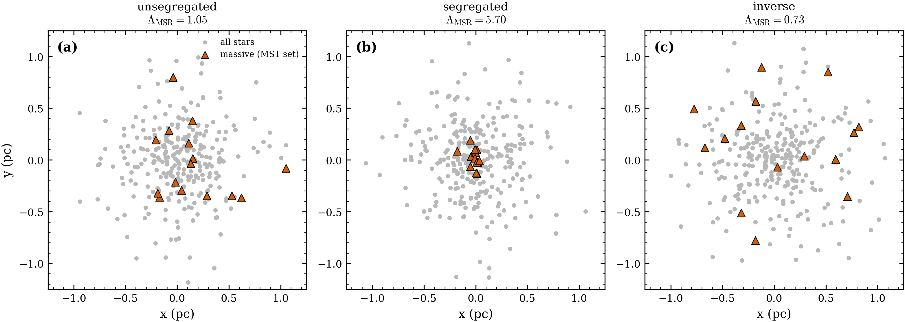
Figure 1: on three hand-constructed regimes with known answers: unsegregated (random masses → ), maximally segregated (massive stars in a tight core → ), and inverse (massive stars on the rim → ). ▲ marks the set whose MST is .
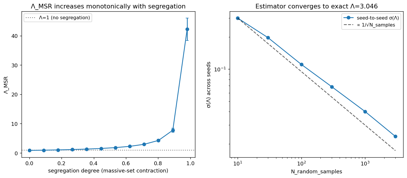
Figure 2:Left: rises monotonically as the massive set is concentrated toward the centre. Right: the estimator converges to the exact value (independent enumeration) with seed-to-seed scatter .
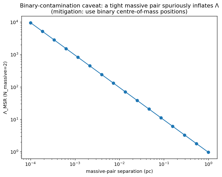
Figure 3:Quantifying the caveat: at a tight massive pair drives , inflating it by 103–104 as the separation shrinks to 10-4 pc. The effect is milder at large (one of edges); mitigation is to use binary centre-of-mass positions.
The implementation lives in progenax.diagnostics.mass_segregation,
which uses scipy’s minimum_spanning_tree and is not part of the
JIT-able core IC pipeline (diagnostics are deliberately kept separate
from the differentiable core; see JAX-native substructure design for
the broader JAX-native-MST design discussion).
Other constructions (not implemented in progenax)
Šubr et al. (2008) parameterise mass segregation via interparticle potential energies rather than total energies — physically equivalent in limit but harder to implement without rejection sampling. progenax adopts only the energy-ordered Baumgardt construction because:
It avoids rejection sampling (deterministic given a fixed orbit pool).
It composes with any equilibrium orbit pool (Plummer, King, EFF, LIMEPY) through the protocol API.
Continuous, differentiable segregation control is already provided by the separate equilibrium route (
MultiComponentCluster.from_mass_segregation), so the primordial generator can stay an honest discrete construction.
The Šubr et al. (2008) construction may be added as an alternative backend in a future version if science needs require it.
Implementation in progenax
Both routes are public in progenax:
import jax
import jax.numpy as jnp
from jaxstro.units import STELLAR
from progenax import (
    MultiComponentCluster,
    PlummerProfile,
    PlummerVelocityDF,
    energy_sorted_segregation,
)
from progenax.profiles import compute_profile_potential

# --- Route 1: equilibrium segregation (differentiable in delta) ---
cluster = MultiComponentCluster.from_mass_segregation(
    alpha_j=jnp.array([0.5, 0.5]),
    m_j=jnp.array([0.3, 1.0]),
    W0=7.0, g=1.0, delta=0.5,
)
ic = cluster.sample_cluster(jax.random.PRNGKey(42), n_stars=1000, G=STELLAR.G)

# --- Route 2: primordial energy-ordered segregation (S = 1) ---
key_pos, key_vel, key_seg = jax.random.split(jax.random.PRNGKey(0), 3)
N, pool_factor = 1000, 4
masses = jnp.ones(N)  # or an IMF draw
pool_masses = jnp.ones(N * pool_factor)
profile = PlummerProfile(r_h=1.0)
df = PlummerVelocityDF(r_h=1.0)
pos_pool = profile.sample_positions(pool_masses, key_pos)
vel_pool = df.sample_velocities(pos_pool, pool_masses, key_vel, G=STELLAR.G)
masses_out, positions, velocities = energy_sorted_segregation(
    key_seg, masses, pos_pool, vel_pool,
    potential_fn=lambda p: compute_profile_potential(
        p, "plummer", jnp.sum(masses), 1.0, STELLAR.G),
)
The primordial sorter implements the discrete energy-ordered assignment and is not itself differentiable; for gradient-based inference over segregation strength use Route 1 ( is the differentiable knob). See Mass segregation validation for the current validation status page.
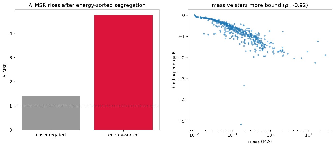
Figure 4:End-to-end check of energy_sorted_segregation (scripts/validate_cluster_ic.py): applying the
energy-ordered assignment to an unsegregated Kroupa-IMF Plummer pool drives the independently
validated from 1.40 to 14.3 (left), and the most massive stars occupy
the most-bound orbits (right, Spearman ) — the construction described above produces
real, -detectable mass segregation.
Relation to fractal substructure
Mass segregation and fractal/clumpy substructure are conceptually
orthogonal pathways, but they live in different packages: turbulent
substructure ICs are the experimental, repo-only gravoturb
package, while both segregation routes are released progenax. Defining
“most bound” orbits inside a strongly clumpy potential is not
implemented anywhere; for most production use cases, choose one of:
Clumpy + subvirial (, experimental
gravoturbICs) — let dynamical segregation emerge during evolution Allison et al., 2009.Smooth + segregated (,
MultiComponentCluster.from_mass_segregationorenergy_sorted_segregation) — primordial segregation in equilibrium.
See Fractal substructure for the substructure side.
Implementation, validation & references
In code: the primordial energy-ordered generator is
energy_sorted_segregationinsrc/progenax/cluster/mass_segregation.py; the differentiable equilibrium route isMultiComponentCluster.from_mass_segregationinsrc/progenax/cluster/multicomponent.py; the diagnostic issrc/progenax/diagnostics/mass_segregation.py. See the cluster API and the diagnostics API.Validated in: mass segregation — the ground-truth suite and the end-to-end generator check; the equilibrium route is additionally pinned by multimass equilibrium.
Primary sources: the energy-ordered construction follows Baumgardt et al. (2008); the partial-segregation -shuffle follows Küpper et al. (2011); the diagnostic is Allison et al. (2009); the equipartition law is Gieles & Zocchi (2015); Šubr et al. (2008) describes the alternative interparticle-energy construction not implemented here. Full notes in the bibliography.
- Allison, R. J., Goodwin, S. P., Parker, R. J., Portegies Zwart, S. F., de Grijs, R., & Kouwenhoven, M. B. N. (2009). Using the minimum spanning tree to trace mass segregation. Monthly Notices of the Royal Astronomical Society, 395, 1449–1454. 10.1111/j.1365-2966.2009.14508.x
- Baumgardt, H., De Marchi, G., & Kroupa, P. (2008). Evidence for primordial mass segregation in globular clusters. The Astrophysical Journal, 685, 247–253. 10.1086/590488
- Küpper, A. H. W., Maschberger, T., Kroupa, P., & Baumgardt, H. (2011). Mass segregation and fractal substructure in young massive clusters. Monthly Notices of the Royal Astronomical Society, 417, 2300–2317. 10.1111/j.1365-2966.2011.19412.x
- Gieles, M., & Zocchi, A. (2015). A family of lowered isothermal models. Monthly Notices of the Royal Astronomical Society, 454, 576–592. 10.1093/mnras/stv1848
- Šubr, L., Kroupa, P., & Baumgardt, H. (2008). A new method to create initially mass segregated star clusters in virial equilibrium. Monthly Notices of the Royal Astronomical Society, 385, 1673–1680. 10.1111/j.1365-2966.2008.12993.x