Classical IMFs¶
The single-star initial mass function captures the birth-mass distribution of individual stars formed in a single star-formation event. It is the standard input for population synthesis, chemical evolution, and the IMF-inference problems progenax is built to solve. Four functional forms dominate the literature, each with a regime where it is the natural choice:
IMF | Class | Use when |
|---|---|---|
Salpeter (1955) |
| Single power law . Use when only the high-mass slope matters and the stellar sample doesn’t reach below . |
Kroupa (2001) |
| 3- or 4-segment broken power-law that captures the low-mass turnover. Standard default for resolved-cluster work. |
Chabrier (2003) |
| Lognormal below matched to a Salpeter-like power-law above. Standard for unresolved-population integrated colours. |
Maschberger (2013) |
| Smooth, three-parameter, analytically invertible IMF. Default for progenax production work because of its closed-form sampling. |
Truncated power-law |
| Hard cutoffs at and . Useful for testing edge cases or modelling stellar populations with explicit upper-mass limits. |
This chapter derives each form, lists the parameter values that turn it into “the” canonical IMF, and explains why progenax picks Maschberger (2013) as its default in production.
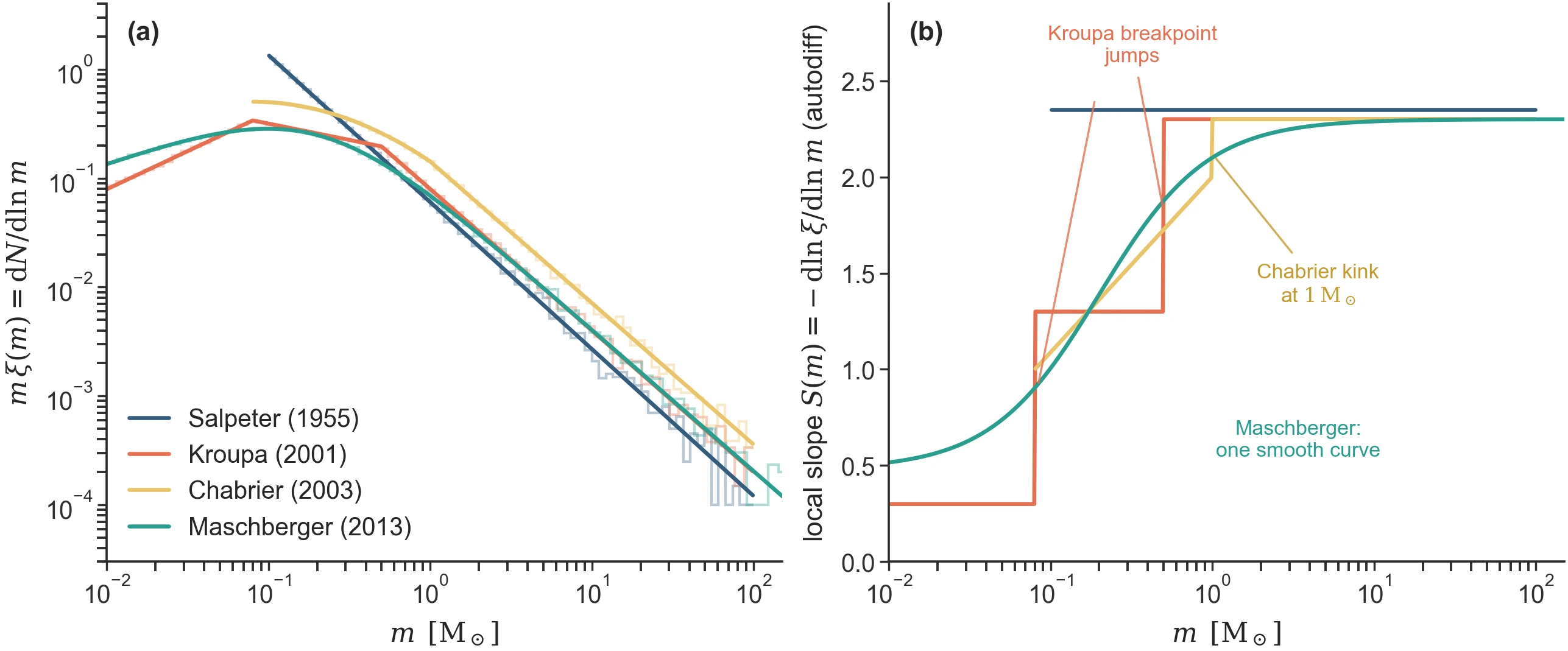
Figure 1:The four classic IMFs and why smoothness matters. (a) for each family on its canonical support
(curves: analytic; faint steps: sampled masses each, seed 42 —
the sampler-equals-theory check). (b) the local slope
computed by autodiff:
Kroupa’s breakpoints and Chabrier’s join are kinks in
exactly the quantity gradient-based inference differentiates through, while
Maschberger is one smooth curve — the reason it is progenax’s production
default. Regenerate: python -m laboratory.icviz --only imf-classic-slopes.
Salpeter (1955): the original power-law¶
The first published IMF, fit to Galactic-disk solar-neighbourhood stars Salpeter, 1955:
valid for . Below the actual stellar distribution turns over (the IMF flattens and eventually decreases toward sub-stellar masses), which Salpeter does not capture. Modern usage typically restricts (1) to and pairs it with a separate low-mass model — which is essentially the Kroupa construction below.
The cumulative is closed-form:
inverted analytically for inverse-CDF sampling. progenax’s
PowerLawIMF.salpeter(m_min=1.0, m_max=150.0) is the Salpeter
configuration (internally exponents=[2.35], breakpoints=[]).
Kroupa (2001): multi-segment broken power-law¶
Kroupa (2001) extends Salpeter to a piecewise broken power-law that captures the observed low-mass turnover:
with continuity coefficients enforced at each break. The four-segment form includes the brown-dwarf regime (); a common three-segment usage drops and starts at . The two high-mass slopes match the Salpeter value (different normalisation conventions account for the small difference between Salpeter’s 2.35 and Kroupa’s 2.3).
PowerLawIMF accepts arbitrary segment slopes and break-points
(breakpoints lists the interior breaks only, excluding m_min and
m_max):
from progenax.imf import PowerLawIMF

# canonical Kroupa: the two equal high-mass slopes (2.3) merge to one
# segment, so the classmethod uses 3 segments / 2 breaks (exact).
kroupa = PowerLawIMF.kroupa(m_min=0.01, m_max=150.0)

# or build the explicit 4-segment form directly:
kroupa4 = PowerLawIMF(
    exponents=[0.3, 1.3, 2.3, 2.3],
    breakpoints=[0.08, 0.5, 1.0],
    m_min=0.01,
    m_max=150.0,
)
The class internally computes the continuity coefficients (so that is continuous at each break) and the per-segment integrals needed for normalisation and sampling.
Chabrier (2003): lognormal + power-law¶
Chabrier (2003) replaces the broken-power-law low-mass piece with a lognormal:
with the Chabrier (2003) Table 1 single-star (disk) values
(0.079), , and
, joined continuously at . (The
often-quoted , are the system IMF;
progenax’s ChabrierIMF defaults to the single-star disk form — its
defaults are m_c=0.08, sigma=0.69, alpha=2.3, m_trans=1.0.) The
lognormal provides a smoother low-mass description than the broken
power-law, which matters for unresolved-population integrated
luminosities and colours. ChabrierIMF is the standard implementation;
it shares its high-mass tail slope with PowerLawIMF.
The Chabrier IMF does not admit a closed-form inverse CDF. Sampling uses a Newton solver on ; the iteration count is fixed at 30 steps which is enough for double-precision convergence across the entire mass range.
Maschberger (2013): smooth and analytically invertible¶
The Maschberger (2013) “L3” form is progenax’s production default because it captures the same physics as Chabrier+Kroupa with a single smooth functional form and a closed-form inverse CDF:
with default parameters (Salpeter slope), , (peak mass). The two factors interact:
For : the second factor approaches 1, leaving the high-mass power-law tail (= Salpeter).
For : the second factor suppresses the distribution, producing the observed turnover below .
The closed-form CDF and its inverse are derived in Maschberger (2013) §3. For ,
with and the
primitive evaluated at the integration endpoints. progenax’s
Maschberger class uses (6) directly, with
no Newton solver, no rejection sampling, fully vmap-compatible.
Check yourself¶
1. The slope trap — reconcile 1.35 with 2.35
Salpeter (1955) reports a slope of 1.35; PowerLawIMF.salpeter() uses
2.35. Before peeking: which convention is which, and how do they relate?
Verify numerically: sample 105 masses, histogram them in , and fit the high-mass tail slope — you should recover (the Jacobian shifts the exponent by one).
2. Rank the mean masses — then explain the outlier
Predict the ordering of for the four default
configurations, then run imf.mean_mass() for each. Measured values
(analytic, this checkout): Salpeter 0.351, Maschberger 0.367, Kroupa
0.376, Chabrier .
The lesson: the biggest driver is the support, not the shape — Chabrier’s default (the hydrogen-burning limit) excludes the brown dwarfs the other defaults include, nearly doubling ; Salpeter’s missing turnover is almost exactly offset by its floor. For a fixed total mass, your IMF choice changes the number of stars by the same factor.
3. Feel the kink with jax.grad
Compute jax.grad(lambda mu: Maschberger(mu=mu).mean_mass())(0.2) — a
clean . Now try
the same through a Kroupa breakpoint (rebuild PowerLawIMF with a traced
break). Both are finite — but relate what you see to panel (b) of
Figure 1: the Maschberger derivative is smooth in
all its parameters everywhere, while a sampled mass sitting exactly at a
Kroupa break feels a kink. Smoothness is why HMC chains on
() mix cleanly.
Truncated power-law¶
TruncatedIMF wraps any of the above with explicit hard cutoffs at
and . This is useful for:
Testing edge cases (e.g. forcing to study a specific stellar regime).
Cluster-mass-dependent upper limits via the Marks et al. (2012) Weidner-Kroupa relation .
Survey selection effects where stars below some completeness threshold are not observed.
The truncation is implemented via inverse-CDF resampling within the truncated range — not by rejection — so all sampled masses are guaranteed inside in a single pass.
Comparison and choice guide¶
IMF | Sampling cost | Continuity | Best for |
|---|---|---|---|
Salpeter | inverse CDF | Power-law only | High-mass-only studies |
Kroupa | per segment | Continuous, breaks at fixed masses | Resolved cluster work; backwards compatibility |
Chabrier | Newton solver | Smooth (lognormal join) | Unresolved-population colours |
Maschberger | inverse CDF | smooth | progenax production default |
Truncated | As above + clamp | As above | Edge cases, |
For new users: use Maschberger unless you have a specific reason to
pick another. For comparison with prior work using a different IMF,
match the convention of the comparison; progenax’s flexible
PowerLawIMF + ChabrierIMF cover the standard alternatives.
Connection to binary-aware and environment IMFs¶
The IMFs above describe single-star distributions. They feed into the binary-aware framework (Binary-aware IMF recovery) where the primary mass is drawn from and the secondary is drawn conditionally from the Moe & Di Stefano (2017) mass-ratio distribution. They also feed into the environment-dependent framework (Environment-dependent IMFs) where the slopes become functions of cloud-core density and metallicity per Marks et al. (2012).
Both extensions wrap the classical IMF rather than replacing it: the single-star remains the underlying object, with binary multiplicity and environment dependence layered on top.
Implementation, validation & references¶
In code:
src/progenax/imf/power_law.py(PowerLawIMF, the Salpeter/Kroupa classmethods),chabrier.py(ChabrierIMF),smooth.py(Maschberger), andtruncated.py(TruncatedIMF) — see the IMF API.Validated in: IMF statistics — the regression suite that checks each sampled distribution against its analytic form.
Primary sources: Salpeter (1955), Kroupa (2001), Chabrier (2003), and Maschberger (2013) — full notes in the bibliography.
- Maschberger, T. (2013). On the function describing the stellar initial mass function. Monthly Notices of the Royal Astronomical Society, 429, 1725–1733. 10.1093/mnras/sts479
- Salpeter, E. E. (1955). The luminosity function and stellar evolution. The Astrophysical Journal, 121, 161–167. 10.1086/145971
- Kroupa, P. (2001). On the variation of the initial mass function. Monthly Notices of the Royal Astronomical Society, 322, 231–246. 10.1046/j.1365-8711.2001.04022.x
- Chabrier, G. (2003). Galactic stellar and substellar initial mass function. Publications of the Astronomical Society of the Pacific, 115, 763–795. 10.1086/376392
- Marks, M., Kroupa, P., Dabringhausen, J., & Pawlowski, M. S. (2012). Evidence for top-heavy stellar initial mass functions with increasing density and decreasing metallicity. Monthly Notices of the Royal Astronomical Society, 422, 2246–2254. 10.1111/j.1365-2966.2012.20767.x
- Moe, M., & Di Stefano, R. (2017). Mind your Ps and Qs: The interrelation between period (P) and mass-ratio (Q) distributions of binary stars. The Astrophysical Journal Supplement Series, 230, 15. 10.3847/1538-4365/aa6fb6