This is the flagship demo: it couples a cluster’s mass function to its internal kinematics through a single physical parameter, and shows that parameter is recoverable from both channels at once.
The self-consistent physics
A multimass LIMEPY cluster Gieles & Zocchi, 2015 is built from an initial mass function. progenax bins the IMF into mass groups; each group has a representative mass and a population weight set by the IMF. Two-body relaxation drives the cluster toward energy equipartition — heavier stars sink and slow down — encoded in the multimass DF by a per-group velocity scale,
with the central-density-weighted mean mass and the equipartition degree Peuten et al., 2017. Real clusters reach only partial equipartition (); the heaviest stars approach while the light stars saturate at an escape-speed ceiling — the Bianchini relation, derived directly from this same DF on the multimass equipartition theory page.
The high-mass IMF slope. The observed masses follow a Maschberger (2013) IMF whose high-mass behaviour is the power law
(full smooth form and characteristic mass: Maschberger (2013)). Here is the coupling that makes the demo self-consistent: the same that sets the slope of the observed mass histogram also sets the masses and weights of the equipartition groups in (1) — so is constrained by the masses (the histogram) and by the kinematics (the group-by-group ). The three recovered parameters are , with the central dimensionless concentration.
The joint likelihood
Two channels, summed (scripts/demo_delta_recovery.py):
The kinematic predictor is the differentiable Engine A multimass oracle rebuilt
from inside the traced loss (the find_alpha_for_masses eigenvalue solve
is differentiable in ); the mass term is the analytic,
normalized Maschberger log-pdf — fully differentiable in .
Inputs and assumptions
The fit recovers three parameters ; the truncation order, the total mass, and the mass range are assumed known. The headline result — that the mass channel pins and breaks the kinematic degeneracy — rests on the clean-mock decoupling described above.
Table 1:Model inputs
Input | Meaning and role | Status (fiducial) |
|---|---|---|
IMF high-mass slope; drives both the mass histogram and the equipartition group masses/weights — the self-consistency hinge. | recovered (2.3) | |
Equipartition degree (); = full equipartition. | recovered (0.4) | |
LIMEPY central concentration. | recovered (5.0) | |
, | Number of IMF mass groups (4); LIMEPY truncation order fixed to the King limit (). | known / fixed |
Measured total cluster mass anchoring the velocity scale — treated as exactly known (see below). | known / fixed (data scalar) | |
mass range, | Maschberger bounds (class bounds = draw bounds, so no truncation correction); in model units. | known / fixed |
, bins, occupancy, quadrature | 105 stars; 16 equal-count radial bins; per-cell occupancy floor | numerical choices |
boxes | expit bounds α , , and — physical, not just numerical: it caps short of the Spitzer-unstable that crashes the ODE. | known/fixed bounds |
MLE / NUTS / bias-grid | 3 dispersed Adam starts (300 steps); NUTS 300+600 (off by default); wrong- grid {1.9…2.7} and robustness truths {1.9,2.3,2.7}. | numerical choices |
Result 1 — joint recovery (freshly run, ALL PASS)
Measured 2026-06-11 (, three dispersed Adam starts; exit 0):
Parameter | Truth | Pull | |
|---|---|---|---|
(IMF high-mass slope) | 2.300 | -1.68 | |
(equipartition degree) | 0.400 | -0.08 | |
(central concentration) | 5.000 | -0.48 |
All within (the heaviest, sparsest group has occupancy , so the fit is not starved). The MLE is a robust optimum — the two best of the three dispersed starts agree in loss to .
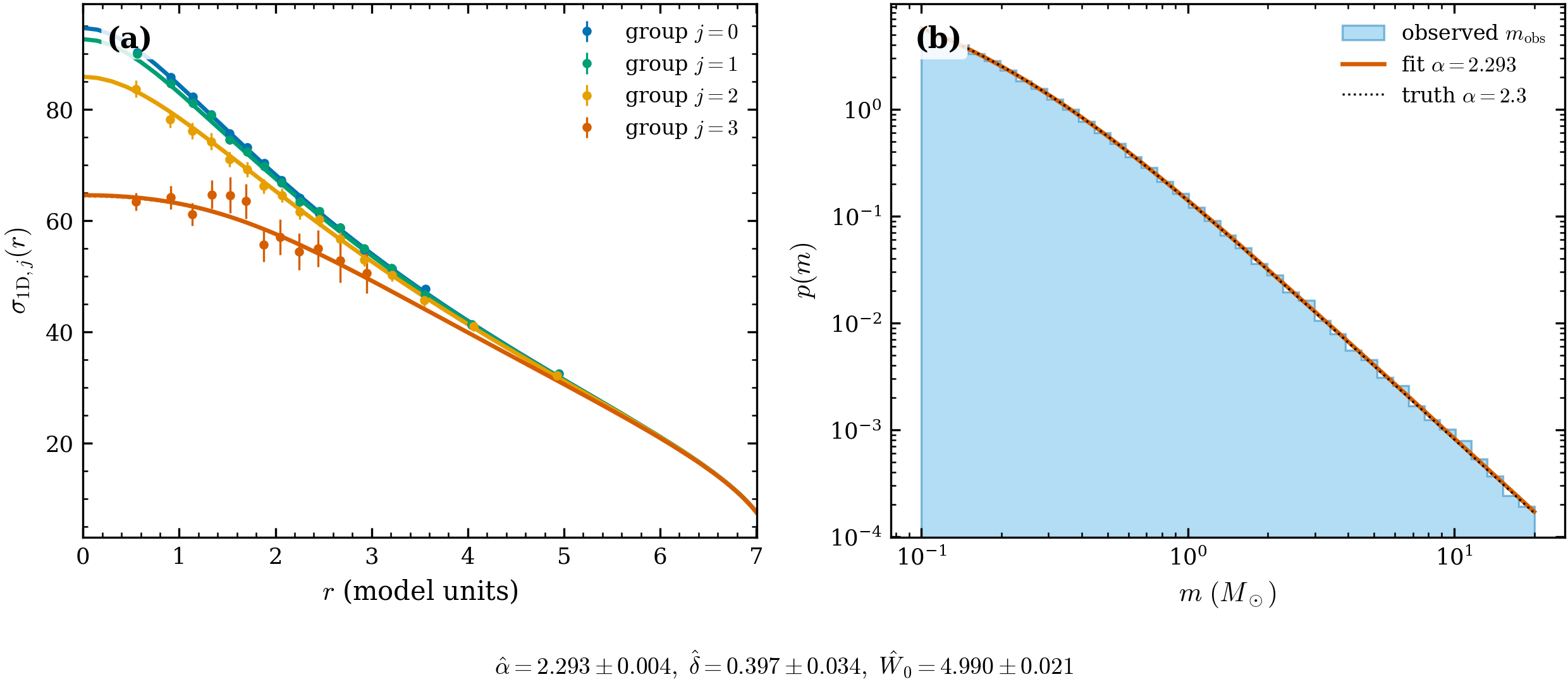
Figure 1:Joint MLE fit (demo_delta_recovery.py). (a) Per-group binned
(points, finite- errors) with the best-fit
binned-expectation curves — the equipartition ordering ( decreasing with
group mass) is visible. (b) The observed mass histogram with the fitted
Maschberger pdf at .
Result 2 — the degeneracy the mass channel breaks
Kinematics alone cannot cleanly separate from : a steeper can come from a larger equipartition degree or from an that reweights the group masses. The Fisher information quantifies it (freshly measured):
Quantity | Kinematics-only | Joint (+ mass channel) |
|---|---|---|
correlation | -0.265 | -0.059 |
0.0192 | 0.0041 | |
0.0357 | 0.0344 | |
ellipse area |
Adding the mass histogram pins tighter (ellipse area ratio 4.67) and collapses the correlation from -0.265 toward zero. Crucially the mass channel pins rather than rotating the ellipse — ’s width barely moves (); the gain is almost entirely in .
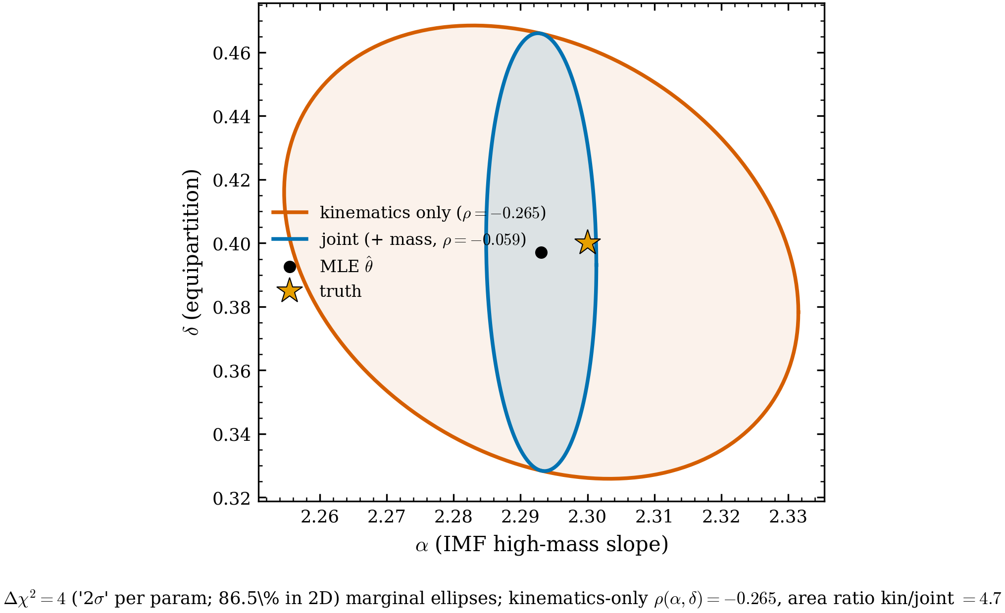
Figure 2:Fisher degeneracy panel. ( in 2-D) ellipses in : the broad, tilted kinematics-only ellipse vs the compact joint ellipse. The mass channel removes the degeneracy along .
Result 3 — full posterior (NUTS)
A vendored blackjax No-U-Turn sampler (300 warmup + 600 samples) draws the full
posterior. Recorded measured run (--run-nuts, min wall):
0 divergent transitions;
posterior mean within of the MLE per parameter (, , );
the target is made flat in by adding the reparametrization Jacobian, so the corner is a faithful posterior, not a box-edge artifact.
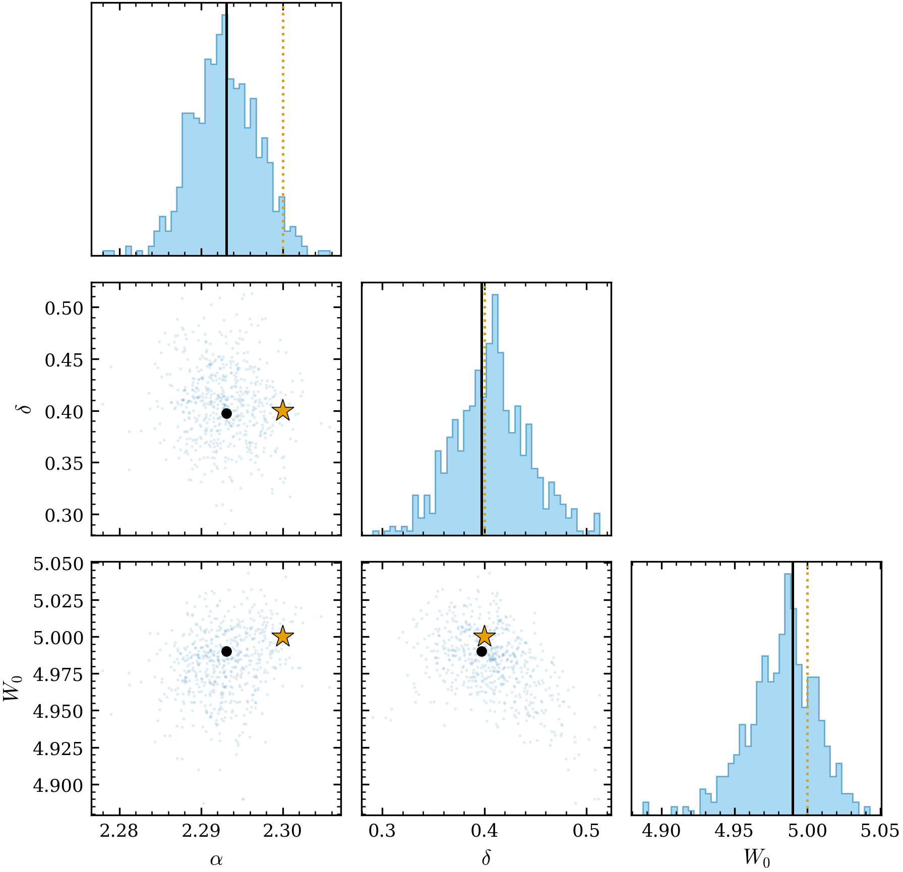
Figure 3:NUTS posterior corner in with the MLE and truth overlaid; unimodal, no divergences, posterior mean on the MLE.
Result 4 — wrong-IMF bias + robustness grid
What if you assume the wrong and refit only the kinematics? Freezing at a grid of wrong values and refitting from kinematics alone (5 seeds each) gives the bias curve. The recovered peaks at the true ( at ) and is biased low on either side — assuming the wrong IMF slope corrupts the equipartition measurement. The linear sensitivity (seed-ensemble SE) is near zero precisely because the response is peaked, not monotonic — it is reported, not gated (no published reference value to assert against).
The companion robustness grid regenerates fresh truth datasets at and refits the full joint — every case recovers within :
max pull | ||||
|---|---|---|---|---|
1.9 | 0.97 | |||
2.3 | 0.51 | |||
2.7 | 0.96 |
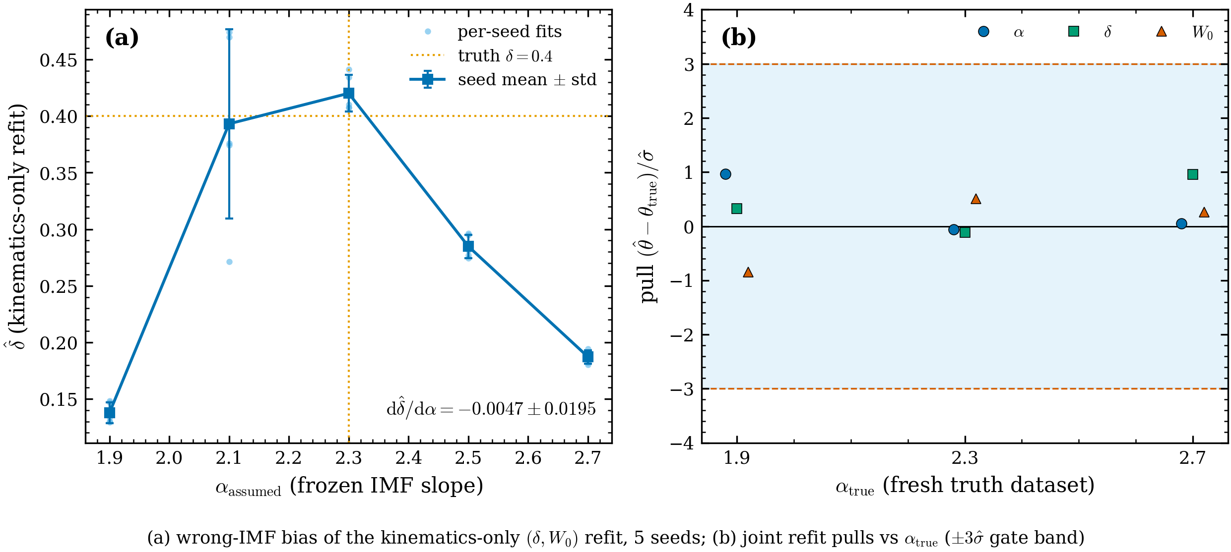
Figure 4:Wrong-IMF bias (left) — with seed scatter, peaking at truth; robustness grid (right) — joint recovery across three , all within .
Caveats
How to run
env -u VIRTUAL_ENV uv run --no-sync python scripts/demo_delta_recovery.py            # MLE + Fisher (minutes)
env -u VIRTUAL_ENV uv run --no-sync python scripts/demo_delta_recovery.py --run-nuts # + NUTS corner (~52 min)
env -u VIRTUAL_ENV uv run --no-sync python scripts/demo_delta_recovery_bias.py # wrong-IMF curve + gridReferences
The multimass LIMEPY DF is Gieles & Zocchi (2015) with the equipartition -convention of Peuten et al. (2017); the equipartition relation and its derived equipartition mass are Bianchini et al. (2016); the IMF is Maschberger (2013). The equipartition physics is developed on the multimass equipartition theory page, and the underlying equilibrium is validated at multimass equilibrium.
- Gieles, M., & Zocchi, A. (2015). A family of lowered isothermal models. Monthly Notices of the Royal Astronomical Society, 454, 576–592. 10.1093/mnras/stv1848
- Peuten, M., Zocchi, A., Gieles, M., Gualandris, A., & Hénault-Brunet, V. (2017). Testing lowered isothermal models with direct N-body simulations of globular clusters – II. Multimass models. Monthly Notices of the Royal Astronomical Society, 470, 2736–2761. 10.1093/mnras/stx1311
- Maschberger, T. (2013). On the function describing the stellar initial mass function. Monthly Notices of the Royal Astronomical Society, 429, 1725–1733. 10.1093/mnras/sts479
- Bianchini, P., van de Ven, G., Norris, M. A., Schinnerer, E., & Varri, A. L. (2016). A novel look at energy equipartition in globular clusters. Monthly Notices of the Royal Astronomical Society, 458, 3644–3654. 10.1093/mnras/stw552