Rotation & the omega-inclination degeneracy (B8)

Rotation & the $\omega$ –inclination degeneracy (B8)¶

The other demos work on clean 3-D mocks. This one takes the first step toward observational realism: a rotating cluster is viewed at an inclination, and the recovered rotation depends on a line-of-sight projection. The honest result is the headline of the realism axis — the mean line-of-sight velocity measures the product $\omega\sin i$ , never the rotation rate $\omega$ alone.

The physics¶

Solid-body rotation about the cluster $z$ -axis gives $\mathbf v = \omega(\hat z \times \mathbf r)$ . The demo’s projection helper project_los tilts the cluster by the inclination $i$ (about the sky $x$ -axis) and reads the line-of-sight (observer $z$ ) velocity. The mean is linear in the sky $x$ -coordinate:

\langle v_{\rm los}\rangle(x_{\rm sky}) = \omega\,\sin i\;x_{\rm sky}.

(1)

A face-on cluster ( $i=0$ ) shows no rotation signature; an edge-on one ( $i=90^\circ$ ) shows the full $\omega$ . So the observable rotation amplitude is the slope $k = \omega\sin i$ . The recovered slope (a clean linear fit of the binned $\langle v_{\rm los}\rangle$ ) is

quantity	truth	recovered
$k = \omega\sin i$	1.732 ( $\omega=2.0$ , $i=60^\circ$ )	$1.69 \pm 0.03$ (pull -1.34)

Inputs and assumptions¶

The fit recovers one observable, the slope $k=\omega\sin i$ — not the rotation rate $\omega$ itself (see the degeneracy). The physical $\omega$ and inclination $i$ are inputs held at truth.

Table 2:Model inputs

Input	Meaning and role	Status (fiducial)
$k=\omega\sin i$	Slope of $\langle v_{\rm los}\rangle$ vs sky- $x$ — what the data actually constrain (`z[0]`).	recovered ( $k_{\rm true}=1.73$ )
$\omega$	Solid-body rotation rate; the physical target, but only the product $\omega\sin i$ is measurable from $\langle v_{\rm los}\rangle$ .	known / fixed (2.0 /Myr); degenerate, not recovered
$i$	Inclination of the spin axis to the line of sight; degenerate with $\omega$ (needs external info, e.g. flattening).	known / fixed ( $60^\circ$ ); degenerate
$r_h$ , spin axis, masses, $G$	Plummer half-mass radius (1 pc); spin axis $=\hat z$ tilted about sky- $x$ only (no position angle); equal-mass tracers; $G$ (STELLAR).	known / fixed
projection model	The assumed linear forward model $\langle v_{\rm los}\rangle = k\,x_{\rm sky}$ from a pure-inclination tilt about one axis.	known / fixed (model assumption)
$N$ , bins, box, MLE, gates	$2\times10^4$ stars; 16 sky- $x$ quantile bins (min 30/bin); slope box $(-20,20)$ ; 3 Adam starts; gates self-consistency $4\sigma$ , recovery $3\sigma$ , degeneracy cond 10⁸.	numerical choices

The degeneracy (the headline)¶

Because $\langle v_{\rm los}\rangle$ depends only on the product, $\omega$ and $i$ are degenerate: $\partial k/\partial(\omega, i) = (\sin i,\ \omega\cos i)$ , so the $(\omega, i)$ Fisher information $\mathcal F = (\nabla k)(\nabla k)^\top/\sigma_k^2$ is rank 1, with eigenvalues

\lambda(\mathcal F) = (8\times10^{-14},\ 1.9\times10^{3}),

(2)

— one machine-precision zero (condition number $\sim 10^{16}$ ). Every $(\omega, i)$ on the curve $\omega = \hat k/\sin i$ fits the line-of-sight velocities equally well (panel c). Recovering the rotation rate needs an independent inclination — e.g. from the projected flattening — which line-of-sight velocities alone cannot supply. This is the same rank-deficient inverse-problem structure as the birth-environment demo, now from projection rather than a many-to-one map.

Figure¶

Rotation & the \omega–i degeneracy (scripts/demo_rotation.py, ALL PASS).
(a) The projected sky map coloured by v_{\rm los}: the rotation dipole —
one side approaching (blue), one receding (red). (b) The rotation curve
\langle v_{\rm los}\rangle(x_{\rm sky}) with the recovered slope k=\omega\sin i.
(c) The degeneracy: every (\omega, i) on \omega=\hat k/\sin i (purple) fits
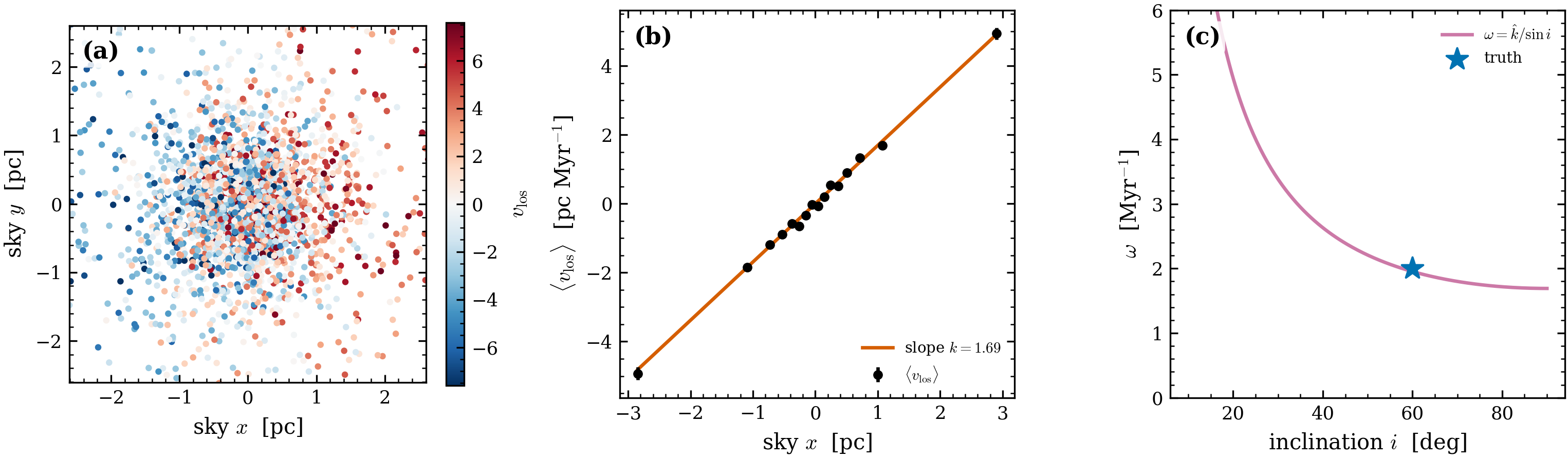
equally well; the truth ★ lies on it. — Figure 1:**Rotation & the $\omega$ – $i$ degeneracy** (`scripts/demo_rotation.py`, ALL PASS). **(a)** The projected sky map coloured by $v_{\rm los}$ : the rotation **dipole** — one side approaching (blue), one receding (red). **(b)** The rotation curve $\langle v_{\rm los}\rangle(x_{\rm sky})$ with the recovered slope $k=\omega\sin i$ . **(c)** The degeneracy: every $(\omega, i)$ on $\omega=\hat k/\sin i$ (purple) fits equally well; the truth ★ lies on it.

Caveats¶

Warning

The bridge, not the destination. This introduces the line-of-sight projection but stops at one realism effect (inclination). Measurement errors, selection / incompleteness, foreground contamination, and a realistic PSF are the rest of the observational-realism arc — applied to all the demos — and are future work.
Solid-body rotation, no anisotropy. A differential rotation curve or a rotation–anisotropy coupling changes $\langle v_{\rm los}\rangle$ ; the degeneracy with $i$ persists but its breaking (via the flattening) is model-dependent.
Clean census, known projection geometry otherwise (the tilt is a pure inclination about one axis; a real cluster also has a position-angle and possibly internal structure).
No velocity measurement noise. Bin standard errors come purely from sampling scatter ( $\mathrm{std}/\sqrt n$ ); there is no per-star RV error $\epsilon$ (the ε-analogue that B12 carries). Stars are also equal-mass tracers, and only the slope is fitted — the systemic velocity and cluster center are assumed known.

How to run¶

env -u VIRTUAL_ENV uv run --no-sync python scripts/demo_rotation.py

References¶

The Plummer model is Plummer (1911); the rotation overlays (apply_solid_body_rotation, apply_differential_rotation) and their non-equilibrium caveats are documented on the rotation & anisotropy page.

References¶

Plummer, H. C. (1911). On the problem of distribution in globular star clusters. Monthly Notices of the Royal Astronomical Society, 71, 460–470. 10.1093/mnras/71.5.460

Rotation & the ω\omegaω–inclination degeneracy (B8)¶

The physics¶

Inputs and assumptions¶

The degeneracy (the headline)¶

Figure¶

Caveats¶

How to run¶

References¶

Rotation & the $\omega$ –inclination degeneracy (B8)¶