King concentration from star counts (B11) - progenax — differentiable initial conditions for N-body simulations

Every other demo in this series recovers structure from the velocity channel $\sigma(r)$ . This one recovers a King King, 1966 cluster’s concentration from the observable a photometric survey actually delivers — the radial star counts — and nothing else. It is the methods showcase for the Poisson number-density channel (binned_number_density / poisson_loglike / poisson_fisher_information).

The physics being recovered¶

A King lowered-isothermal model is fixed by two structural parameters:

$W_0$ — the dimensionless central potential (concentration). It sets the shape of the number-density profile in units of the core radius and the truncation ratio, summarized by the King concentration $c = \log_{10}(r_t/r_c)$ .
$r_c$ — the core radius, the physical scale at which the profile breaks.

So binned counts $N_k$ constrain both: the profile shape pins $W_0$ , the physical break radius pins $r_c$ . The forward model is Engine A — a single King-limit LIMEPY component Gieles & Zocchi, 2015 ( $g=1$ ): the coupled Poisson ODE gives $\psi(r/r_c)$ , and the King volume density is the closed form

\hat n(r) = E_\gamma\!\left(g + \tfrac32,\, W(r)\right), \qquad W(r) = \psi(r/r_c),

(1)

(limepy_density_hat), differentiable in $(W_0, r_c)$ through psi_grid. Beyond $r_t$ the potential $W\le 0$ and the density is exactly zero — the hard truncation that pins the outer profile, and the regime where the Poisson model (honest counting errors on low-occupancy bins) matters most.

The likelihood¶

The expected counts are $\mu_k(W_0, r_c) = N_{\rm obs}\, p_k$ , with $p_k$ the fraction of the model’s enclosed number in radial bin $k$ (the number-weighted integral of $4\pi r^2\,\hat n(r)$ over the bin). The data are the frozen counts; gradients flow through the model only. The per-bin Poisson log-likelihood is $\sum_k\left(N_k\log\mu_k - \mu_k\right)$ . The Fisher information is the reverse-mode Poisson form $J^\top\mathrm{diag}(1/\mu)\,J$ (poisson_fisher_information): the Engine A diffrax solve carries a custom_vjp, so jax.hessian would crash — exactly the constraint that makes the B2 demo use Gauss–Newton.

Inputs and assumptions¶

The fit recovers two parameters $(W_0, r_c)$ from star counts alone; the concentration $c=\log_{10}(r_t/r_c)$ is derived at the solution, not separately fit. Everything else is an assumed-known input or a numerical choice.

Table 1:Model inputs

Input	Meaning and role	Status (fiducial)
$W_0$	Dimensionless central potential (concentration); sets the profile shape and $r_t/r_c$ . A science target.	recovered (6.0)
$r_c$	Core radius — the physical break scale. The second science target.	recovered (1.0 pc)
$c=\log_{10}(r_t/r_c)$	King concentration — reported at the MLE, derived from $(W_0,r_c)$ , not independently fit.	derived
$g$	LIMEPY truncation index fixed to the King limit.	known / fixed (1.0)
$N$ , $G$	Stars sampled / Poisson normalization ( $3\times10^4$ ); gravitational constant (STELLAR) for the sampling.	known / fixed
bins, $r_{\rm lo}$ , $N_{\rm fine}$ , boxes	20 log-spaced count bins; inner edge 0.10 pc (excludes the flat core); 3000-pt enclosed-number integration grid; sigmoid boxes $W_0\in(3.5,7.5)$ (capped — the ODE hits `max_steps` above $\sim$ 8), $r_c\in(0.3,3.0)$ .	numerical choices
$N_{\rm inits}$ , Adam, gates, seeds	3 dispersed Adam starts (400 steps, lr 3e-2); gates self-consistency $4\sigma$ , recovery $3\sigma$ ; seeds (data / inits).	numerical choices

Important

The count channel alone carries a strong $W_0$ – $r_c$ degeneracy ( $\rho=-0.91$ ): a more concentrated model ( $W_0\uparrow$ ) with a smaller core ( $r_c\downarrow$ ) reproduces nearly the same radial count profile. The counts pin both parameters only because the data carry two distinct features — the profile shape pins $W_0$ and the physical break radius pins $r_c$ — with most of the $W_0$ leverage coming from the low-occupancy outer bins (the hard truncation at $r_t$ , where the density is exactly zero). This is why the per-bin Poisson likelihood (not a Gaussian on counts) is essential: it gives those near-empty outer bins honest weight. The marginals stay tight ( $\lesssim2\%$ ), but the parameters are far from independent; breaking the correlation needs the velocity channel $\sigma(r)$ , which this count-only demo deliberately omits.

Result — freshly run, ALL PASS¶

Measured 2026-06-12 ( $N=3\times10^4$ stars, $K=20$ log-spaced bins over $[0.10, 16.8]$ pc, three dispersed Adam starts; wall $\approx 29$ s; exit 0).

Parameter	Truth	$\hat\theta \pm \hat\sigma$	Pull
$W_0$ (concentration)	6.000	$6.028 \pm 0.024$	+1.15
$r_c$ (core radius)	1.000 pc	$0.995 \pm 0.010$ pc	-0.47

Both within $1.2\sigma$ . Supporting diagnostics, same run:

King concentration recovered. $c = \log_{10}(r_t/r_c) = 1.263$ at the MLE vs 1.255 at truth — the model’s $c(W_0)$ relation is validated against King (1966) Table II on the King validation page.
Robust optimum. All three dispersed initializations converged to the identical loss $-2.02978\times10^{5}$ .
Self-consistency. The analytic prediction at truth matches the binned counts to $\max|N_k-\mu_k|/\sqrt{\mu_k} = 2.51$ over the 20 bins — no oracle/binning bias.

The honest catch: counts alone are degenerate¶

The Gauss–Newton Fisher correlation is $\rho(W_0, r_c) = -0.91$ . The number-density profile alone leaves a strong $W_0$ – $r_c$ degeneracy: a more concentrated model ( $W_0\!\uparrow$ ) with a smaller core ( $r_c\!\downarrow$ ) reproduces almost the same count profile over the binned range. Both marginals are still tight (the demo recovers each to $\lesssim 2\%$ ), but the parameters are far from independent — the $2\sigma$ Fisher ellipse is a thin diagonal sliver (panel b). This is precisely the degeneracy the velocity channel breaks: $\sigma(r)$ adds the gravitational-mass / velocity-scale information that counts cannot supply, which is why the multi-channel demos (B2, B3) pin their parameters far more tightly. B11 isolates what the count channel can and cannot do on its own.

Figure¶

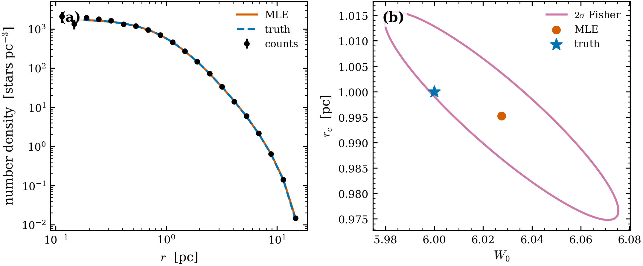
$King concentration from star counts (scripts/demo_king_concentration.py, ALL PASS). (a) The radial number-density profile: binned counts per shell volume (points, \sqrt N errors) with the best-fit (vermilion) and truth (blue dashed) King profiles, across the core-to-truncation dynamic range. (b) The 2\sigma Fisher ellipse in (W_0, r_c): a thin diagonal sliver (\rho=-0.91) — the strong count-channel degeneracy — with the truth ★ inside, near the MLE.$

Figure 1:King concentration from star counts (scripts/demo_king_concentration.py, ALL PASS). (a) The radial number-density profile: binned counts per shell volume (points, $\sqrt N$ errors) with the best-fit (vermilion) and truth (blue dashed) King profiles, across the core-to-truncation dynamic range. (b) The $2\sigma$ Fisher ellipse in $(W_0, r_c)$ : a thin diagonal sliver ( $\rho=-0.91$ ) — the strong count-channel degeneracy — with the truth ★ inside, near the MLE.

Caveats¶

Warning

Clean mock, single family. Truth and fit are the same Engine A King model; the data are 3-D radial counts with no projection, completeness, or contamination. This isolates the count-channel inference, not observational recovery.
Counts alone are degenerate ( $\rho(W_0,r_c)=-0.91$ ). The point of B11 is to show this, not hide it; breaking the degeneracy needs the velocity channel.
Inner 0.1 pc excluded. The flat King core inside the first bin edge ( $0.1\,r_c$ , $\sim$ 0.1% of the mass) is dropped from the fit; the normalization is over the binned range.
$W_0$ box capped at 7.5. Above $W_0\sim 8$ the Engine A diffrax solve hits its step limit; the fit is bounded to the safe range (truth 6 is well interior). The $r_c$ box $(0.3,3.0)$ is a bound of the same kind.
3-D radial counts, not projected. The demo bins true 3-D radii; a real survey delivers the projected surface-density profile (an Abel-related but distinct observable), which this demo does not model.
Single realization. One seed (SEED=0) draws the data; the headline pulls and uncertainties are from a single mock (not an ensemble), and the outer bin edge is data-dependent ( $\min(r_{\max},r_t)$ ), a minor reproducibility subtlety.

How to run¶

env -u VIRTUAL_ENV uv run --no-sync python scripts/demo_king_concentration.py

References¶

The King lowered-isothermal model is King (1966); the LIMEPY family and the $g=1$ King limit are Gieles & Zocchi (2015). The Engine A construction and its $c(W_0)$ validation against King (1966) Table II are documented on the populations and physics-tests pages.

References¶

King, I. R. (1966). The structure of star clusters. III. Some simple dynamical models. The Astronomical Journal, 71, 64–75. 10.1086/109857
Gieles, M., & Zocchi, A. (2015). A family of lowered isothermal models. Monthly Notices of the Royal Astronomical Society, 454, 576–592. 10.1093/mnras/stv1848