A real cluster is not one population. This demo builds a two-family cluster — a spatially extended, kinematically anisotropic halo plus a compact, isotropic core — in one shared self-consistent potential, and asks whether three structural parameters can be recovered jointly from its kinematics:
— the halo mass fraction (the core carries ),
— the halo’s Osipkov-Merritt anisotropy radius,
— the halo’s Plummer half-mass radius.
The truth model (the science-headline mix of the Engine B validation suite):
sampled with stars. The EFF core shape , the stellar-mass labels , and the core’s isotropy are held fixed; only are recovered.
The physics being recovered
Anisotropy (Osipkov-Merritt). The halo’s DF depends on energy and angular momentum only through , which makes the velocity ellipsoid isotropic in the centre and increasingly radial outside . The Binney anisotropy has the closed form
so as (isotropic) and as (radial). The core, with , has . The OM curve Merritt, 1985 is the second observable, and it is what pins .
Dispersion. The 1-D dispersion of each component is built from the speed moments of its Eddington DF in the shared potential, with the OM stretch folded in:
where are the stretched-frame speed moments. This is the verbatim oracle the Engine B validation suite checks against sampled velocities. Physical units come from the engine’s own velocity scale , anchored to the measured total mass (never an input ).
Why and together recover all three. The halo scale sets where falls off; the mass split sets the relative amplitude and shape of the two components’ dispersion profiles; is read almost entirely from the rising . The three are nearly orthogonal — borne out by the near-zero Fisher correlations below.
Inputs and assumptions
The fit recovers three halo parameters ; the core family, the domain radius, and the total mass are all assumed known. The split matters: the recovery looks clean partly because the hardest potential degeneracy ( vs the cluster’s outer extent) is removed by fixing the domain.
Table 1:Model inputs
Input | Meaning and role | Status (fiducial) |
|---|---|---|
Halo (Plummer) mass fraction; core carries . Read from the relative dispersion amplitudes. | recovered (0.6) | |
Halo Osipkov–Merritt anisotropy radius; read from the rising . | recovered (3.0 pc) | |
Halo Plummer half-mass radius; sets where falls off. | recovered (2.0 pc) | |
core EFF , isotropy | Fixed core density profile ( pc, ) and isotropic core () — not fitted. | known / fixed |
Domain outer radius = the fixed EFF extent, passed explicitly so a traced never re-derives the boundary. | known / fixed (9.0 pc) | |
Stellar-mass labels [halo 0.5, core 1.0] ; the cancels in the per-bin ratio. | known / fixed | |
Measured total mass anchoring the physical velocity scale — treated as exactly known (see below). | known / fixed (data scalar) | |
, bins, occupancy, quadrature, MLE | stars; 16 equal-count radial bins; occupancy floors | numerical choices |
Result — joint MLE + Fisher (freshly run, ALL PASS)
Measured 2026-06-11 (, three dispersed Adam starts; exit 0):
Parameter | Truth | Pull | |
|---|---|---|---|
(halo mass fraction) | 0.600 | +0.22 | |
(halo OM radius) | 3.000 pc | pc | +0.96 |
(Plummer half-mass) | 2.000 pc | pc | +0.51 |
All three within , comfortably inside the recovery gate. Supporting diagnostics, all measured in the same run:
Robust optimum. All three dispersed initializations converged to the identical loss 19.1479 — the recovered minimum is not an initialization artifact.
Realizability. Rebuilding Engine B at gives DF positivity margins , both — the recovered model is a genuine equilibrium, not a negative-DF fiction.
Self-consistency. The analytic prediction at truth matches the binned data to over all 48 populated cells — no systematic oracle/binning bias.
Near-orthogonality. Gauss-Newton Fisher correlations , (condition number 13.4): the three parameters are independently constrained.
Figure
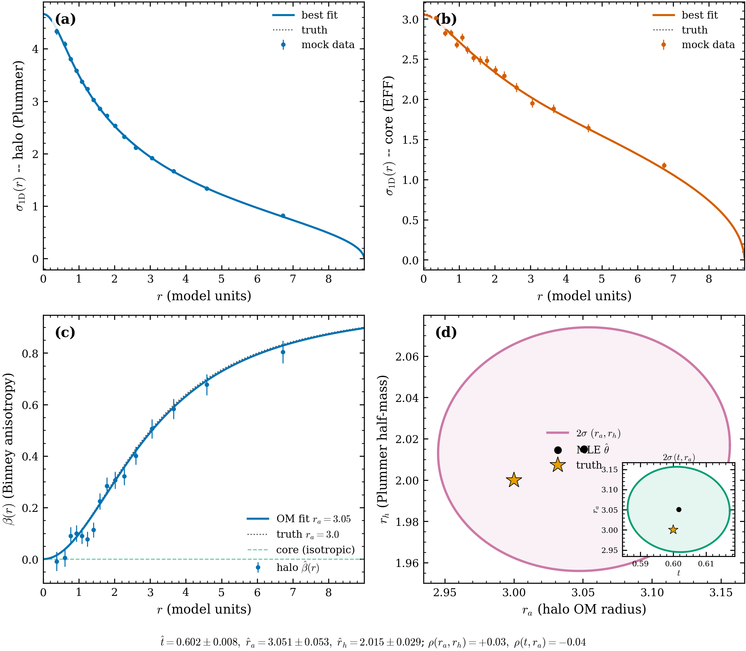
Figure 1:Halo + core recovery (scripts/demo_halo_core.py, ALL PASS). (a, b)
Per-component : mock data (points, finite- error bars)
with the best-fit binned-expectation curve and the truth curve, for the Plummer
halo and EFF core. (c) Halo Binney anisotropy rising along the
OM curve ( pc vs truth 3.0), with the
isotropic-core reference at . (d) Fisher ellipses in
(and inset ): the truth ★ sits inside, near the MLE; the
ellipses are nearly axis-aligned, reflecting the near-zero correlations.
Caveats
How to run
env -u VIRTUAL_ENV uv run --no-sync python scripts/demo_halo_core.pyReferences
The EFF profile is Elson et al. (1987); the Plummer model Plummer (1911); Osipkov-Merritt anisotropy Merritt (1985); Eddington inversion follows Binney & Tremaine (2008). The Engine B construction and its realizability/anisotropy validation are documented at Engine B (Eddington) and the multi-component theory pages.
- Merritt, D. (1985). Spherical stellar systems with spheroidal velocity distributions. The Astronomical Journal, 90, 1027–1037. 10.1086/113810
- Elson, R. A. W., Fall, S. M., & Freeman, K. C. (1987). The structure of young star clusters in the Large Magellanic Cloud. The Astrophysical Journal, 323, 54–78. 10.1086/165807
- Plummer, H. C. (1911). On the problem of distribution in globular star clusters. Monthly Notices of the Royal Astronomical Society, 71, 460–470. 10.1093/mnras/71.5.460