A star cluster’s dynamical mass is read off its velocity dispersion, . But an unresolved binary contributes its orbital motion to the measured velocity, widening the dispersion and biasing the mass high. In low-dispersion systems — ultra-faint dwarfs, low-mass globular clusters — the binary motion is a large fraction of itself, so the bias is large and has driven real debates about mass-to-light ratios and dark-matter content.
This demo (a) quantifies the bias, (b) shows a dispersion-only analysis cannot remove it — the problem is rank-1 degenerate — and (c) demonstrates a differentiable joint recovery from the non-Gaussian wings of the velocity distribution that returns an unbiased dynamical mass, with a Fisher/CRLB forecast vs sample size and RV precision .
It is the kinematic companion to B4: B4 recovers the binary fraction photometrically (from the unresolved-binary mass function); B12 measures the dynamical mass kinematically in the presence of the same binaries. Both reuse the Moe & Di Stefano (2017) –– statistics Moe & Di Stefano, 2017 and the Tout et al. (1996) ZAMS mass–luminosity relation Tout et al., 1996.
The forward model
Each star has a cluster centre-of-mass line-of-sight velocity . A fraction are unresolved binaries: you measure one blended velocity, not two. The blend sits at , where is the internal orbital motion projected onto the line of sight and flux-weighted by the two components’ luminosities,
with the Tout (1996) ZAMS relation (in-package via
progenax.stellar). Two limits make intuitive:
(equal mass): and , so the blend cancels, . Twins are nearly invisible contaminants.
(extreme ratio): the faint secondary adds no light, so you see the primary’s reflex, (an SB1).
The orbits are drawn from the Moe coupling; periods become semimajor axes via Kepler’s third law, and the orbit is sampled at a uniform mean anomaly (uniform in time, so eccentric orbits are correctly weighted toward slow apocenter passages). The distribution of over a large binary pool is the contamination kernel — crucially independent of , so the observed velocity density factorizes,
where is the per-star RV precision (added in quadrature). Because
does not depend on , it is precomputed once.
The expected binned counts
are differentiable in both parameters, and are recovered
by a per-bin Poisson MLE (scripts/_demo_inference.py), with the Fisher from the
Poisson information.
Inputs and assumptions
The fit recovers only two parameters, ; every other quantity is an assumed-known input. Making that split explicit is essential — the demo’s optimism lives entirely in what it treats as known.
Table 1:Model inputs
Input | Meaning and role | Status (fiducial) |
|---|---|---|
Intrinsic cluster LOS velocity dispersion; the science target — sets the dynamical mass . | recovered (5 km/s) | |
Unresolved binary fraction (the contamination weight in (2)). | recovered (0.5) | |
Per-star RV measurement precision (spectrograph noise), added in quadrature to both mixture components. Distinct from (gravity) and (orbits). | known / fixed (1 km/s) — see Important | |
Metallicity for the Tout ZAMS used to flux-weight the blend ((1)). | known / fixed (10-3) | |
Number of RV stars; sets the Poisson normalization and the precision floor (, Figure 5). | known / fixed (1500) | |
Half-mass radius; enters only the conversion, not the velocity-distribution fit. | known / fixed (30 pc) | |
IMF | Maschberger (, 0.08–): draws primary masses , hence and the shape of . | known / fixed |
Moe ––, | The orbital statistics (, period, eccentricity coupling) that define . | known / fixed |
| Likelihood bin edges ( km/s, 120 bins of 1 km/s); must span the wings (next section). | numerical choice |
grid / pool | Template grid km/s and pool size (sets template noise). | numerical choice |
Result — freshly run, ALL GATES PASS
UFD-like regime: km/s, , RV stars, km/s, metal-poor , pc (exit 0; wall s).
Gate | Expected | Measured |
|---|---|---|
1 — bias exists | 1.28 ( km/s) | |
2 — dispersion-only degenerate | rank-1 (cond ) | cond |
3a — joint recovery unbiased | , | , |
3b — full-distribution full-rank | cond | cond |
4 — RV-precision floor | precision degrades, mass unbiased | : ; |
5 — null () | , | |
6 — AD-vs-FD gradient integrity | rel-err |
The bias, and why dispersion-only cannot fix it
The dispersion grows by the variance budget , so the naive virial mass is biased high by exactly — at (Figure 2). Crucially, this is a systematic: averaging more stars at fixed measures the wrong mass more precisely, it does not remove the bias.
A dispersion-only analysis sees a single number , so any on the curve fits equally well — an infinite ridge (Figure 3, orange). Its Fisher is the outer product of one gradient: exactly rank-1 (one zero eigenvalue, cond ). One number cannot separate two unknowns.
How the wings break the degeneracy
The fix is to fit the whole shape of , not just its width. The Gaussian core constrains one combination of ; the non-Gaussian wings — the heavy tail no single-star Gaussian can mimic (Figure 1) — constrain a different combination. Two independent constraints turn the open ridge into a closed ellipse (Figure 3, blue): the full-distribution Fisher is full-rank (cond , a 1013 improvement). The recovered mass is unbiased, km/s, vs the naive 1.28 (verified unbiased over 24 realizations: , ).
The RV-precision floor
Because is known and folded into (2), the recovered mass stays unbiased at every (Figure 4) — even at km/s . What degrades is precision: doubles as washes out the wing signature, and the detectable binary fraction collapses from 0.21 to 0.02. The honest scope: you can only correct for the binaries you can detect, and that detectable fraction shrinks as the spectrograph gets noisier — but the correction you do make is unbiased. The Fisher forecast (Figure 5) shows both uncertainties fall as ; (and hence the bias correction) is the harder parameter, since the wings it lives in are sparsely populated.
Figures
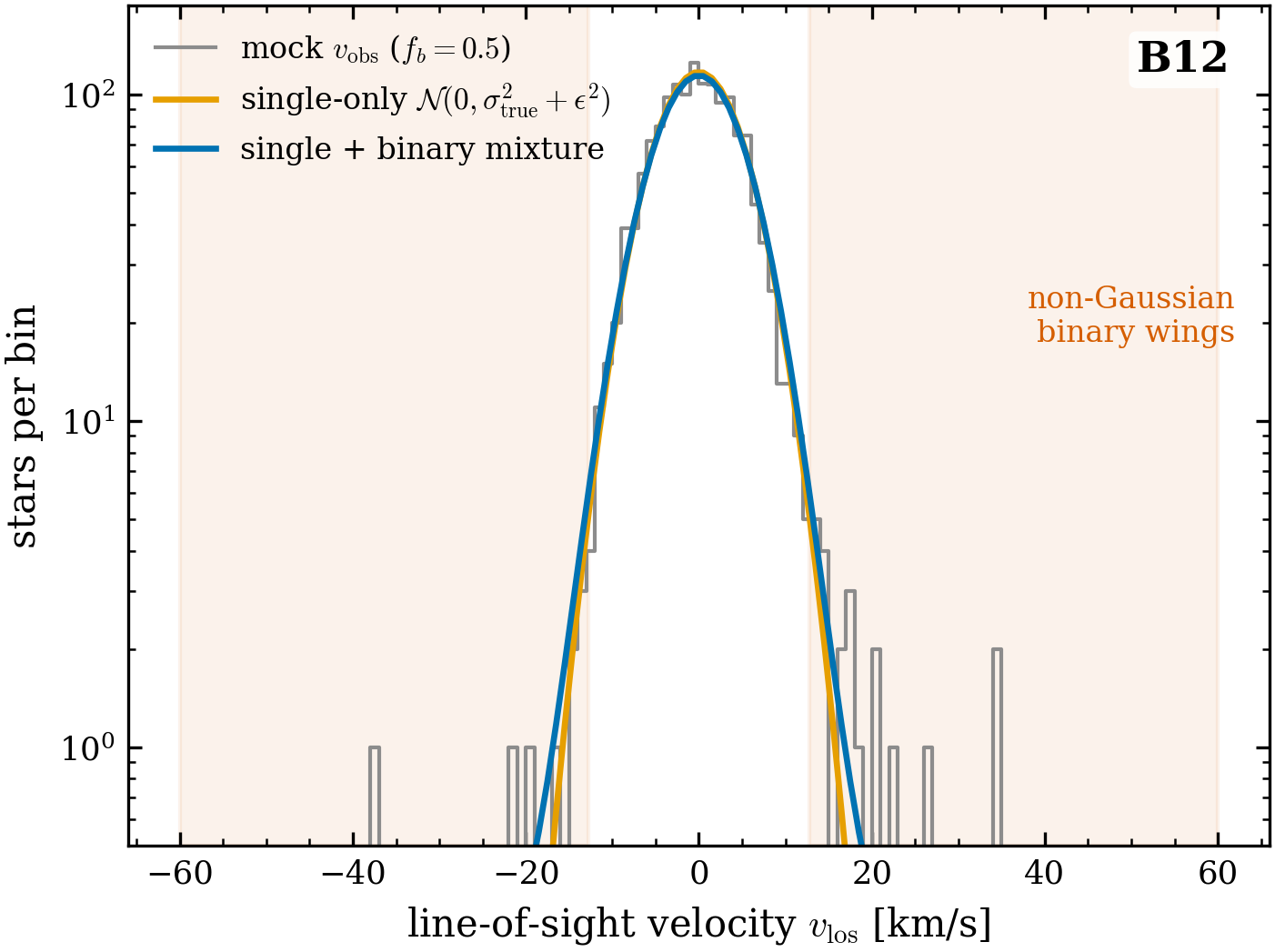
Figure 1:The non-Gaussian wings (log-). The mock (grey) and the single+binary mixture (blue) follow the binary wings out to km/s, where the single-only Gaussian (orange) predicts essentially nothing. The shaded regions () are where the binary excess lives — the signal the joint fit uses to break the degeneracy.
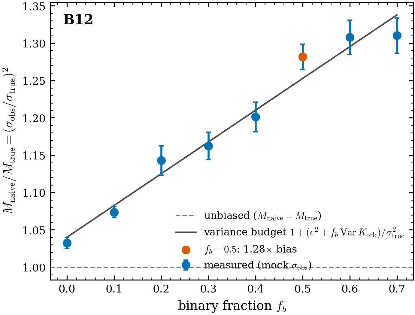
Figure 2:The bias. vs binary fraction (points, 20 realizations each) tracks the analytic variance budget (line). At the virial mass is biased high.
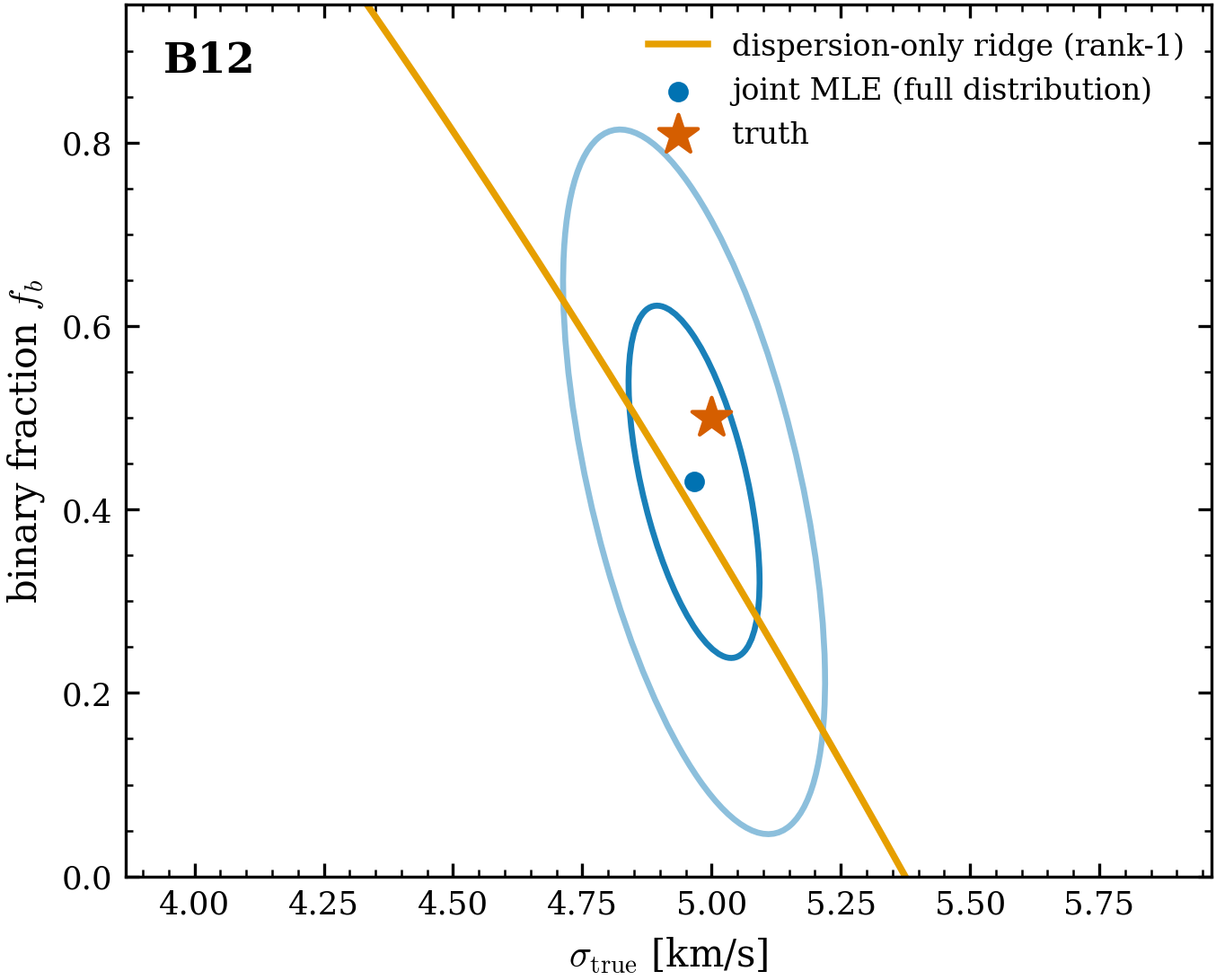
Figure 3:Degeneracy and its breaking. A dispersion-only analysis constrains only the degenerate ridge (orange) — every point gives the same . The full velocity distribution localizes both parameters to the finite 1/ ellipses (blue); truth (star) sits on the ridge and inside the ellipse. The ellipse is elongated along the ridge — the residual correlation the wings only partially lift.
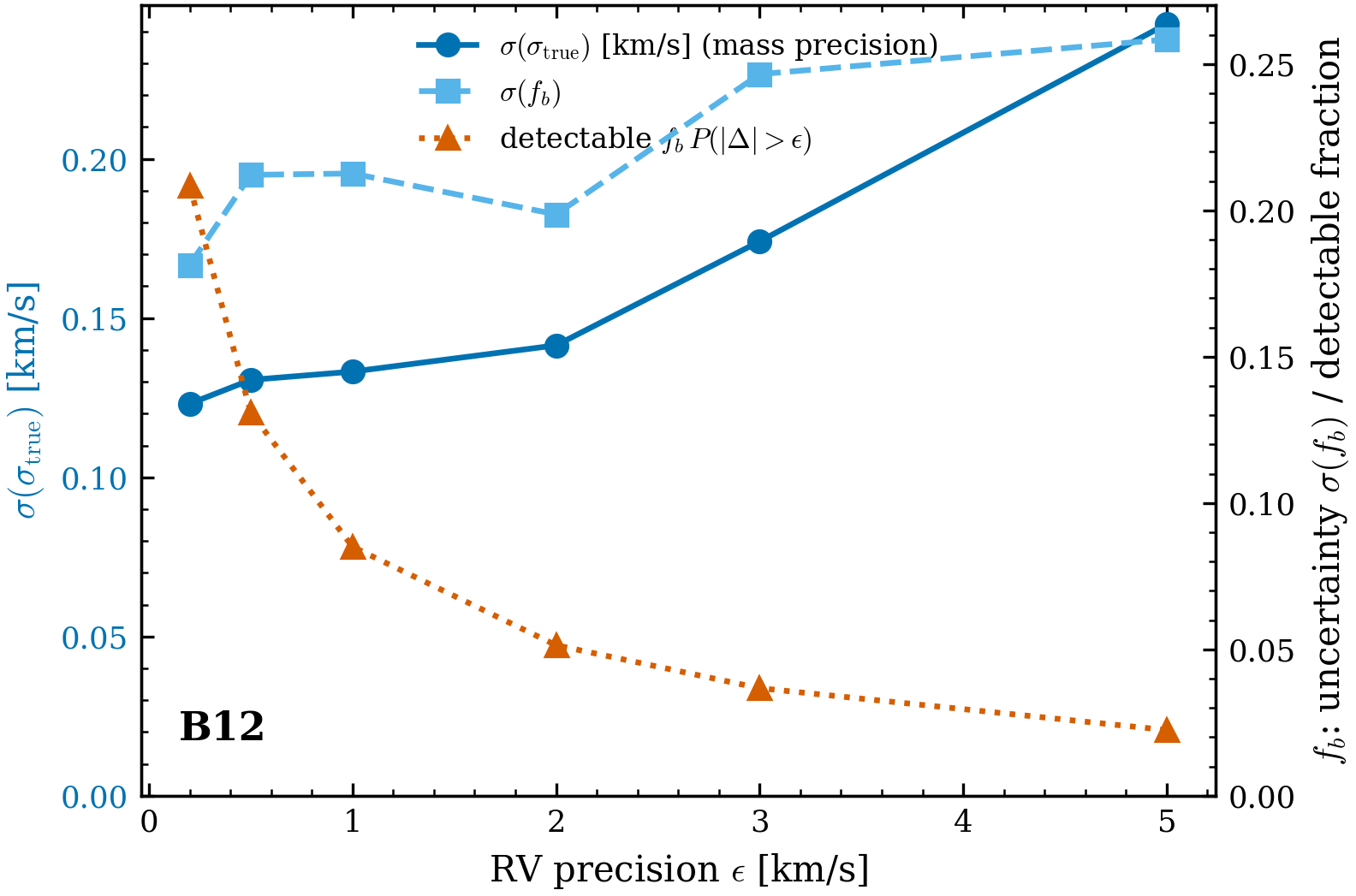
Figure 4:The RV-precision floor. The recovered-mass precision (blue, left) and (sky, right) grow with RV precision , while the detectable fraction (vermilion, right) collapses. The mass itself stays unbiased () at all — only the precision degrades.
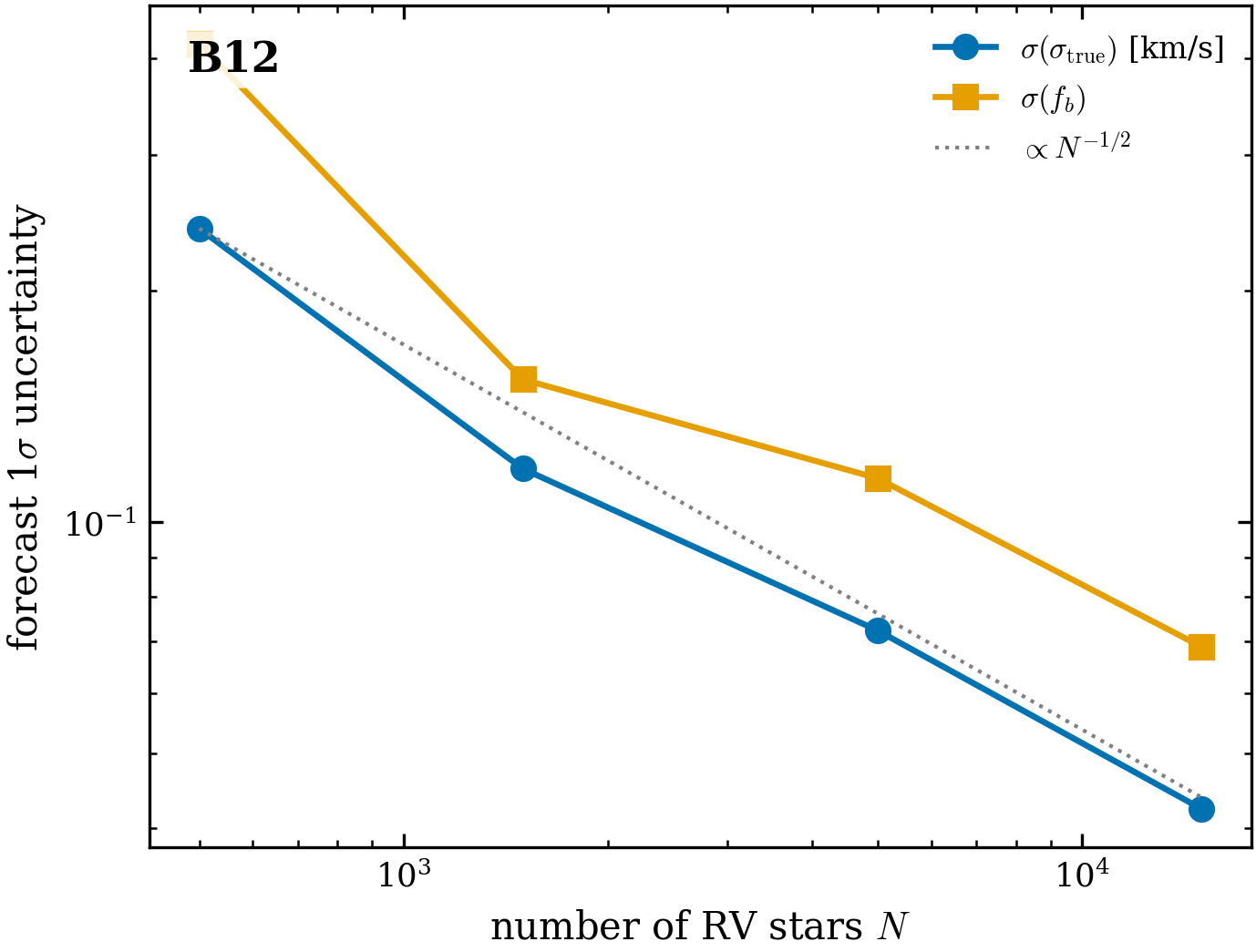
Figure 5:Survey forecast. Fisher and vs sample size (log–log), both scaling as (dotted guide). Small- sits above the guide — the few-star regime is more degenerate than the asymptotic CRLB.
Caveats
How to run
env -u VIRTUAL_ENV uv run --no-sync python scripts/demo_binary_dynamical_mass.pyReferences
The binary –– coupling is Moe & Di Stefano (2017); the ZAMS mass–luminosity relation is Tout et al. (1996). The Moe and companion models are documented on the binary statistics theory pages; the photometric sibling is B4.
- Moe, M., & Di Stefano, R. (2017). Mind your Ps and Qs: The interrelation between period (P) and mass-ratio (Q) distributions of binary stars. The Astrophysical Journal Supplement Series, 230, 15. 10.3847/1538-4365/aa6fb6
- Tout, C. A., Pols, O. R., Eggleton, P. P., & Han, Z. (1996). Zero-age main-sequence radii and luminosities as analytic functions of mass and metallicity. Monthly Notices of the Royal Astronomical Society, 281, 257. 10.1093/mnras/281.1.257