The default equilibrium velocity DFs in progenax — Plummer, King, EFF — are spherical, isotropic, and non-rotating. Real star clusters are often not: globular clusters show modest radial anisotropy in their outer regions King, 1966, young massive clusters frequently rotate, and post-merger or tidally-stressed systems can have substantial velocity anisotropy in either direction.
progenax extends each isotropic DF with two compositional layers:
Osipkov-Merritt radial anisotropy — a one-parameter (, the anisotropy radius) generalisation that makes the velocity ellipsoid radially biased outside and stays isotropic within.
Rotation — solid-body or differential, applied as an additive tangential velocity on top of the isotropic base.
The two layers attach differently: anisotropy is intrinsic to the DF
(an anisotropy_radius constructor argument on PlummerVelocityDF /
EFFVelocityDF), while the rotation overlays are plain functions applied
to the already-sampled (velocities, positions) arrays (or declared via
RotationParams in the pipeline). The composition is order-independent (anisotropy
modifies the velocity ellipsoid; rotation adds a bulk flow), so the
final IC has the right profile and the right rotation
curve.
Osipkov-Merritt anisotropy¶
The Osipkov-Merritt construction replaces the energy-only DF with a DF that depends on the augmented integral
where is the specific angular momentum and is the anisotropy radius. The DF — constructed by Eddington-style inversion using the augmented density — produces a velocity ellipsoid whose anisotropy is
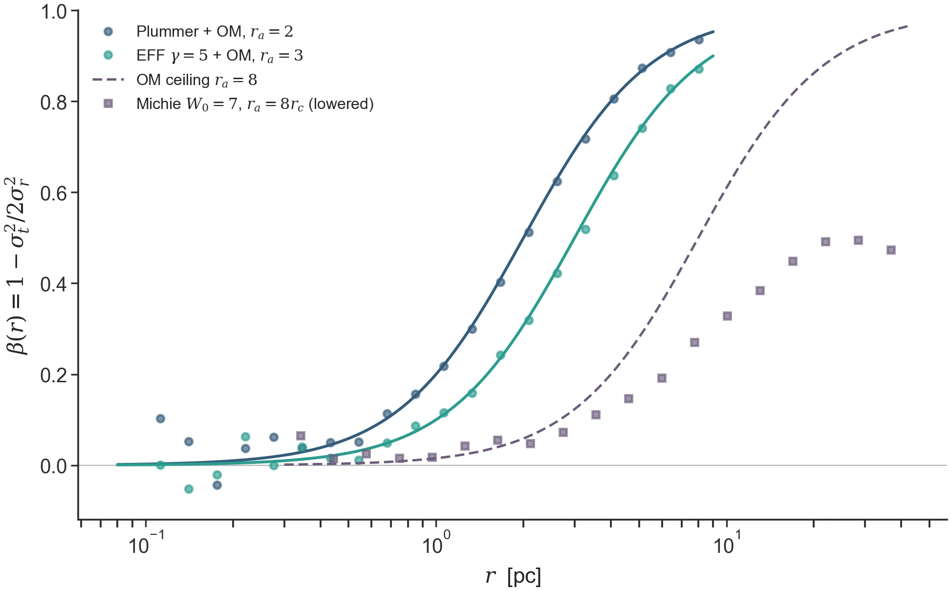
Figure 1:Anisotropy machinery, measured ( per model, seed 12).
OM-Plummer and OM-EFF realized sit on the exact identity
(curves); the self-consistent Michie model (squares) rises
along, then saturates visibly below its OM ceiling (dashed) with a
truncation-edge dip — the lowering removes the most-radial high-energy
orbits, so a lowered model can never reach the pure OM limit. Regenerate:
python -m laboratory.icviz --only beta-anisotropy.
Three regimes:
Velocity ellipsoid | ||
|---|---|---|
Isotropic () | ||
0.5 | Moderately radial | |
Fully radial () |
The anisotropy radius is the only new parameter. Setting recovers the isotropic base DF; setting produces fully radial orbits at all radii (which is generally unphysical and unstable).
Implementation: the anisotropy_radius DF parameter¶
Osipkov-Merritt anisotropy is an intrinsic property of the velocity DF:
pass anisotropy_radius () to a DF. None (default) gives the
isotropic DF; a float gives the radially anisotropic OM DF for the
same density.
from jaxstro.units import STELLAR
from progenax.kinematics import PlummerVelocityDF, EFFVelocityDF

# r_a in the same length units as r_h / a
om_plummer = PlummerVelocityDF(r_h=1.0, anisotropy_radius=2.0)
# gamma=5 reduces EFF to Plummer, so this OM-EFF starts in clean equilibrium
# (Q ~ 0.5). A steep gamma=3 EFF, strongly truncated, is a few percent
# sub-virial even before anisotropy — see the EFF chapter.
om_eff = EFFVelocityDF(a=1.0, gamma=5.0, r_t=10.0, anisotropy_radius=2.0)

velocities = om_plummer.sample_velocities(positions, masses, key, G=STELLAR.G)
Internally (Merritt 1985):
Build from the augmented density — the closed-form Eq. 45 for Plummer, the numerical Eddington inversion of for EFF. The potential is unchanged (set by the true mass density).
At each radius sample a speed from by inverse-CDF — the same machinery as the isotropic DF.
Split isotropically in the stretched frame , then un-stretch the tangential component, which realises exactly.
The DF is JIT-compatible and differentiable in (and /).
Check yourself¶
1. Read off a curve
The OM identity gives exactly. Read the two OM models’ off Figure 1 by finding where each curve crosses — you should recover and 3.
2. Why does Michie sit below its OM ceiling?
Both constructions use the same weight — so why
do the squares saturate near instead of climbing to the
dashed curve? (The King-style lowering removes the highest-energy orbits, and
at large radii those are precisely the most radial ones an OM model relies
on; near the DF empties entirely and dips. The validation
suite pins this ordering: test_beta_below_osipkov_merritt_ceiling.)
Solid-body rotation¶
The simplest rotation prescription adds a tangential velocity to the isotropic base velocities, where is a constant angular-velocity vector (typically aligned with the cluster’s -axis). The resulting per-particle velocity is
This adds a bulk-rotation kinetic-energy contribution
with the moment of inertia perpendicular to .
Because solid-body rotation adds only tangential velocity, the
random-motion velocity dispersion is preserved — but the total
kinetic energy increases, which means the resulting cluster is
supervirial by . You can rescale the speeds to a
target via virial_scale after rotation is applied,
but note the source module’s own warning: a uniform speed rescale does
not restore stationarity — it cannot remove the injected angular
momentum , so a rotation-overlaid IC is a deliberately rotating,
non-stationary initial condition.
from progenax import PlummerProfile, PlummerVelocityDF, virial_scale
from progenax.kinematics import apply_solid_body_rotation

profile = PlummerProfile(r_h=1.0)
df = PlummerVelocityDF(r_h=1.0)
positions = profile.sample_positions(masses, key_pos)
velocities = df.sample_velocities(positions, masses, key_vel, G=STELLAR.G)

# Overlay: add the streaming component v_rot = omega x r. The overlays are
# plain FUNCTIONS on (velocities, positions) arrays — not DF wrappers.
velocities = apply_solid_body_rotation(
    velocities, positions, omega=0.5, axis=jnp.array([0.0, 0.0, 1.0])
)

# Optional: rescale speeds to a target Q_vir (returns the scaled velocities).
# CAVEAT: the uniform rescale cannot remove the injected L_z — the rotating
# IC is deliberately NON-STATIONARY (see kinematics/rotation.py's docstring).
velocities = virial_scale(positions, velocities, masses, Q_target=0.5, G=STELLAR.G)
Differential rotation¶
Differential rotation generalises (3) by allowing to depend on position:
progenax implements a peaked rotation curve in cylindrical radius :
which is solid-body (, constant) in the core, reaches exactly at , and decays exponentially outward — no rotation at the centre or in the far outskirts, the shape observed in rotating globular clusters. (An earlier revision of this page described a user-supplied power-law callable; the shipped API takes the two scalars below.)
from progenax.kinematics import apply_differential_rotation

velocities = apply_differential_rotation(
    velocities, positions, v_peak=0.5, R_peak=1.0,
    axis=jnp.array([0.0, 0.0, 1.0]),
)
The overlay is a plain function on the sampled (velocities, positions)
arrays, fully vmap/JIT-compatible and differentiable in
and (both are grad-audited
registry cases).
Composability¶
Anisotropy is intrinsic to the DF; rotation and an optional virial rescale are layered by the velocity pipeline:
from progenax.kinematics import (
    PlummerVelocityDF, VelocityModel, RotationParams, sample_velocities_pipeline,
)

model = VelocityModel(
    df=PlummerVelocityDF(r_h=1.0, anisotropy_radius=2.0),   # radial anisotropy
    rotation=RotationParams(solid_body=True, pattern_speed=0.3),
)
velocities = sample_velocities_pipeline(key, positions, masses, model, G=STELLAR.G)
The DF sets the velocity ellipsoid (, ); rotation adds a bulk flow on top without changing the random-motion dispersions.
Domain of validity¶
Osipkov-Merritt non-negativity. progenax refuses an below the Plummer bound (Merritt 1985, Eq. 46) at construction (raises
ValueError), and EFF rejects an that drives negative. Even above the bound, very small is prone to the radial-orbit instability within a relaxation time under evolution.Solid-body rotation up to is physically reasonable. Above that, the cluster flattens significantly and a spherical IC is a poor approximation.
Differential-rotation profiles must be smooth — discontinuities in produce delta-function torques on the cluster and non-equilibrium starting states. If your science requires a sharp transition (e.g. a rotating core embedded in a non-rotating envelope), use a smooth-blend rather than a step function.
Implementation, validation & references¶
In code: the rotation overlays live in
src/progenax/kinematics/rotation.py(apply_solid_body_rotation,apply_differential_rotation); the Osipkov–Merritt anisotropy is an intrinsic option on the DFs insrc/progenax/kinematics/(plummer_df.py,eff_df.py). See the kinematics API.Validated in: OM / rotation anisotropy — the realised , the non-negativity bound, and the rotation-curve recovery.
Primary sources: the Osipkov–Merritt construction is Merritt (1985) (the closed-form Plummer bound is Eq. 46); textbook context is Binney & Tremaine Galactic Dynamics §4, and the rotation prescriptions follow the N-body initialisation literature Aarseth et al., 1974Küpper et al., 2011. For a self-consistent rotating King extension, the lowered-model family Gieles & Zocchi (2015) is the natural route (see the lowered-model family), not yet implemented. Full notes in the bibliography.
- King, I. R. (1966). The structure of star clusters. III. Some simple dynamical models. The Astronomical Journal, 71, 64–75. 10.1086/109857
- Merritt, D. (1985). Spherical stellar systems with spheroidal velocity distributions. The Astronomical Journal, 90, 1027–1037. 10.1086/113810
- Aarseth, S. J., Henon, M., & Wielen, R. (1974). A comparison of numerical methods for the study of star cluster dynamics. Astronomy and Astrophysics, 37, 183–187.
- Küpper, A. H. W., Maschberger, T., Kroupa, P., & Baumgardt, H. (2011). Mass segregation and fractal substructure in young massive clusters. Monthly Notices of the Royal Astronomical Society, 417, 2300–2317. 10.1111/j.1365-2966.2011.19412.x
- Gieles, M., & Zocchi, A. (2015). A family of lowered isothermal models. Monthly Notices of the Royal Astronomical Society, 454, 576–592. 10.1093/mnras/stv1848