Spatial density profiles - progenax — differentiable initial conditions for N-body simulations

A spatial density profile $\rho(r)$ is one of the three orthogonal ingredients in every progenax IC (What is an initial condition?). progenax ships four spatial profiles — the isotropic Plummer / King / EFF plus the self-consistent anisotropic Michie–King. They do not share a single size parameter: Plummer is parameterised by the half-mass radius $r_h$ ; King and Michie–King by the central potential $W_0$ and core radius $r_c$ (Michie–King adds the anisotropy radius $r_a$ ); and EFF by the scale radius $a$ , outer slope $\gamma$ , and truncation radius $r_t$ . Convert between the conventions using each profile’s own $r_h$ relation (e.g. (3)) when you need cross-profile comparability.

Profile	$\rho(r)$ form	Use when
Plummer profile	$\rho(r) = \frac{3 M}{4\pi a^3}\,\bigl[1 + (r/a)^2\bigr]^{-5/2}$	You want a smooth, untruncated profile and a closed-form everything (mass, potential, velocity dispersion, distribution function).
King profile	Lowered isothermal sphere; ODE-defined, parameterised by central potential $W_0$ .	You want a tidally truncated cluster matching observed Galactic globular clusters; need a finite outer radius.
EFF profile	$\rho(r) = \rho_0\,\bigl[1 + (r/a)^2\bigr]^{-\gamma/2}$	You want power-law outer falloff matching young massive cluster surface brightness; need a free outer-slope parameter.
Michie-King anisotropic model	Self-consistent King with a Gaussian-in- $J^2$ anisotropy term (Michie 1963); ODE-defined, distinct from isotropic King.	You want a tidally-truncated cluster with radial velocity anisotropy increasing outward (the Michie–King model). Density and DF are solved together.

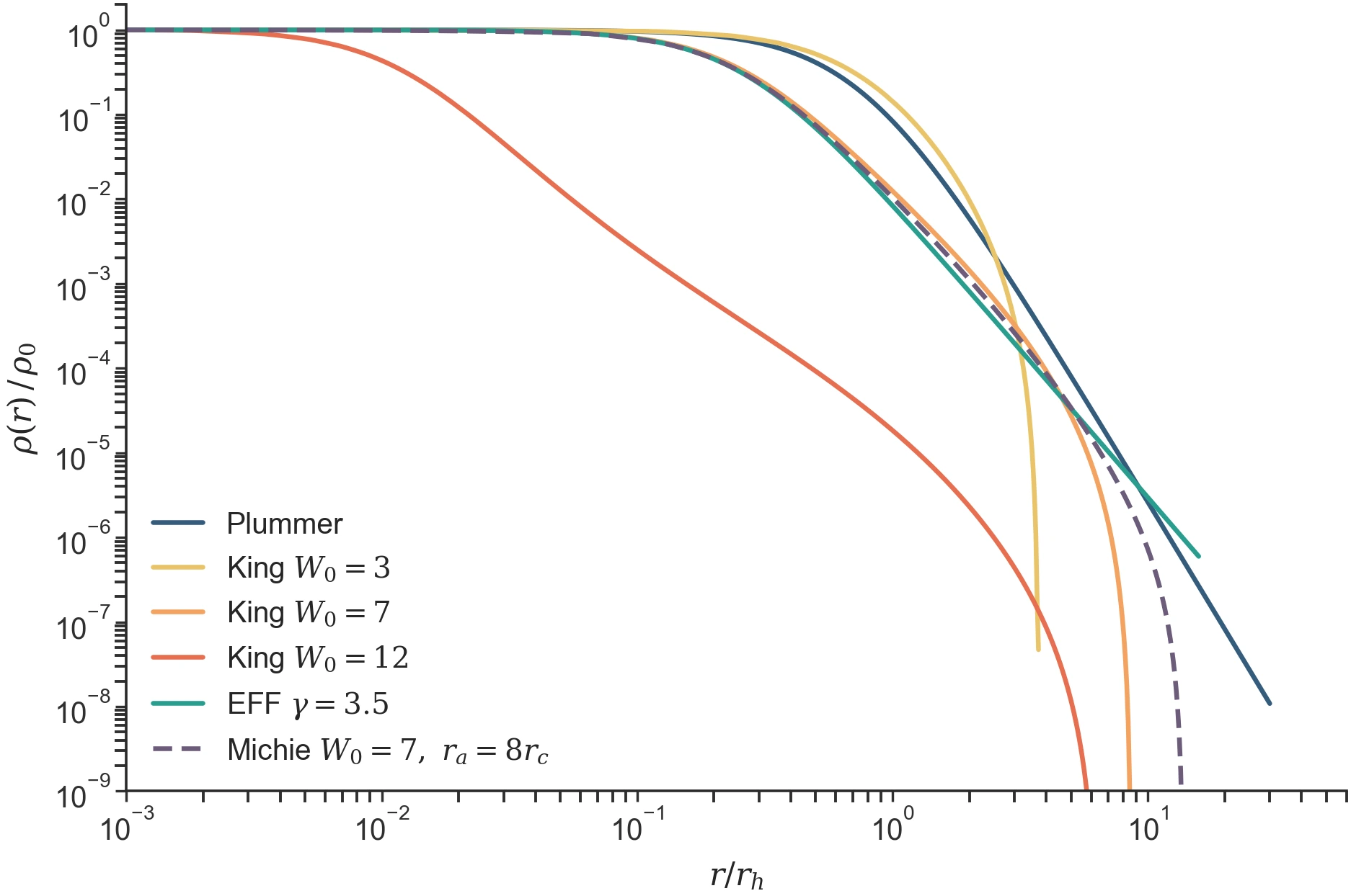
$The model-selection table, drawn: every released density family, half-mass-normalized. Plummer’s untruncated r^{-5} tail; the King W_0 = 3 \to 12 sequence (each \sim4–5 units of W_0 buys a decade of core-to-tidal contrast c = \log_{10} r_t/r_c: 0.67 \to 1.53 \to 2.74); EFF’s shallow power-law halo crossing Plummer at large radii; Michie (dashed) as “King, but more extended” — radial anisotropy visible as pure structure. Regenerate: python -m laboratory.icviz --only profile-family-portrait.$

Figure 1:The model-selection table, drawn: every released density family, half-mass-normalized. Plummer’s untruncated $r^{-5}$ tail; the King $W_0 = 3 \to 12$ sequence (each $\sim$ 4–5 units of $W_0$ buys a decade of core-to-tidal contrast $c = \log_{10} r_t/r_c$ : $0.67 \to 1.53 \to 2.74$ ); EFF’s shallow power-law halo crossing Plummer at large radii; Michie (dashed) as “King, but more extended” — radial anisotropy visible as pure structure. Regenerate: python -m laboratory.icviz --only profile-family-portrait.

Plummer is the default (closed-form everything). King fits old, tidally truncated globulars ( $W_0 \sim 5$ –9); EFF fits young massive clusters whose power-law halos King’s exponential edge cannot capture Elson et al., 1987; Michie–King adds self-consistent radial anisotropy to the King picture.

Common API contract¶

Every spatial profile satisfies the SpatialProfile protocol (Protocol-based composition):

class SpatialProfile(Protocol):
    def sample_positions(
        self,
        masses: Float[Array, "N"],
        key: PRNGKey,
    ) -> Float[Array, "N 3"]:
        """Draw N positions from ρ(r). Returns (N, 3) Cartesian."""
        ...

    def characteristic_radius(self) -> Float[Array, ""]:
        """A representative scale (r_h for Plummer, r_t for King/EFF),
        used e.g. for softening defaults."""
        ...

The protocol’s contract is just these two methods — there is no shared r_h field and no density/cumulative_mass requirement (the concrete classes provide density where it is closed-form, e.g. Plummer and EFF, but the protocol does not mandate it). sample_positions uses an inverse-CDF sampler over a fixed grid so that the positions themselves are differentiable in the size parameter ( $r_h$ for Plummer, $r_c$ / $W_0$ for King, $a$ / $\gamma$ for EFF) — useful when the loss function depends on post-sampling spatial moments.

Composability with velocity DFs and modifiers¶

Each profile pairs with a matching equilibrium velocity DF for in-equilibrium ICs:

Profile	Equilibrium velocity DF	Out-of-equilibrium pairing?
Plummer	`progenax.kinematics.PlummerVelocityDF` (Plummer velocity distribution functions)	Plummer + isothermal velocity → cold-collapse IC
King	`progenax.kinematics.KingVelocityDF` (King velocity distribution functions)	King + Plummer DF → mismatched IC for testing relaxation
EFF	`progenax.kinematics.EFFVelocityDF`	EFF + isotropic-Maxwellian → approximate but useful starting state
Michie–King	`progenax.kinematics.MichieVelocityDF` (Michie-King anisotropic model)	Solved self-consistently as a pair (`MichieProfile` + `MichieVelocityDF`); the density is intrinsic to the anisotropic DF

All four profiles compose with the modifier layers — mass segregation (Mass segregation), fractal substructure (Fractal substructure), and tidal truncation (Tidal physics) — without changing the underlying $\rho(r)$ .

Sampler fidelity at a glance¶

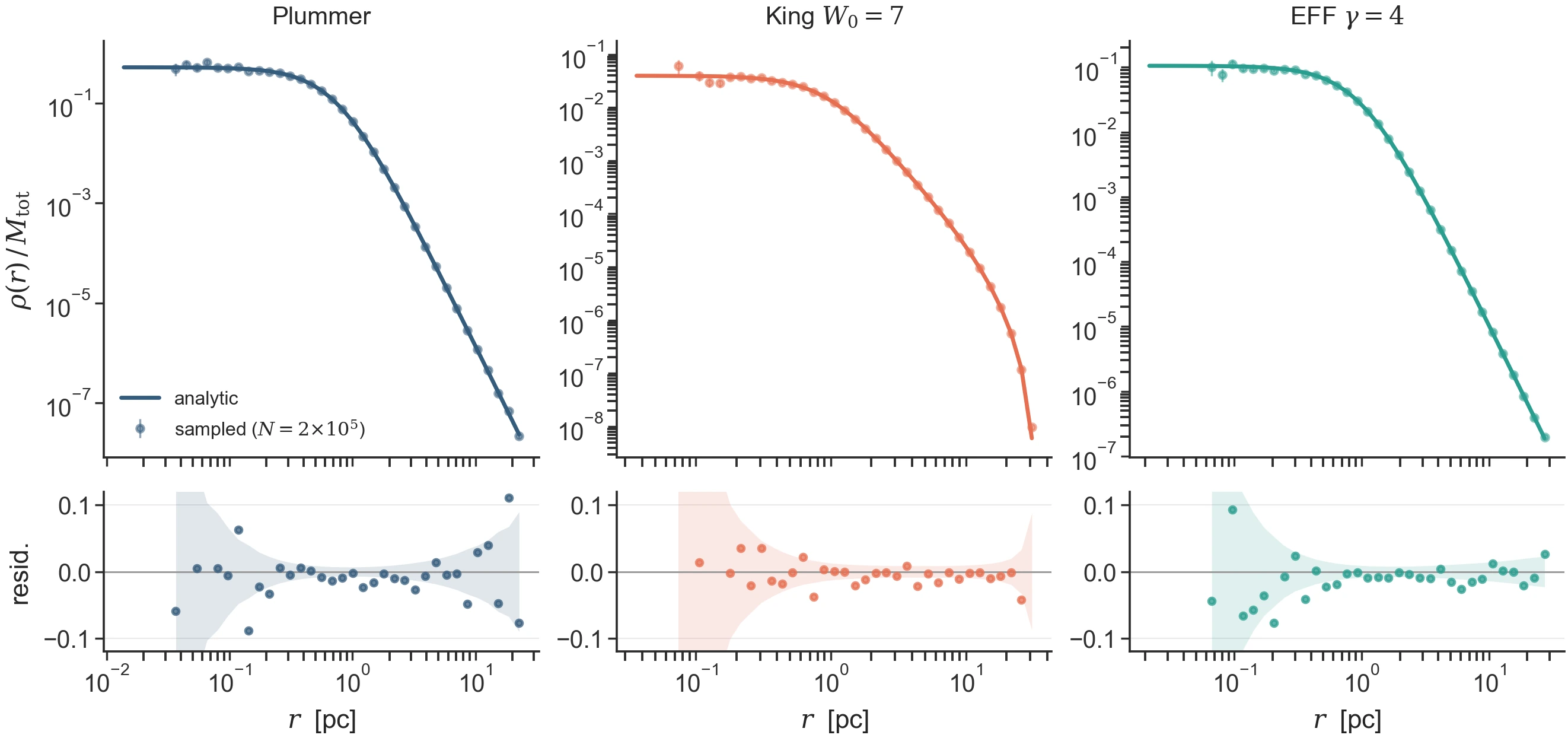
$Sampled radial densities (N = 2\times 10^5 per family, seed 7) against the analytic curves, spanning 6–7 decades, with residuals inside the \pm 1/\sqrt{N_{\rm bin}} Poisson bands (shaded). Bins with fewer than 10 stars are dropped. Quantitative gates: Plummer, King, EFF. Regenerate: python -m laboratory.icviz --only profile-density-residuals.$

Figure 2:Sampled radial densities ( $N = 2\times 10^5$ per family, seed 7) against the analytic curves, spanning 6–7 decades, with residuals inside the $\pm 1/\sqrt{N_{\rm bin}}$ Poisson bands (shaded). Bins with fewer than 10 stars are dropped. Quantitative gates: Plummer, King, EFF. Regenerate: python -m laboratory.icviz --only profile-density-residuals.

Check yourself¶

Implementation, validation & references¶

In code: the profiles live under src/progenax/profiles/ (plummer.py, king.py, eff.py, michie.py) with their paired DFs under src/progenax/kinematics/. See the profiles API and the kinematics API; the per-profile theory pages (Plummer, King, EFF) carry the exact module paths.
Validated in: Plummer, King, EFF, and Michie anisotropy.
Primary sources: the isotropic profiles are Plummer (1911), King (1966), and Elson et al. (1987); the anisotropic Michie–King model is Michie (1963) (+ King (1966) cutoff). The lowered-model family Gieles & Zocchi (2015) unifies these under a single multi-mass family that progenax implements natively (see the lowered-model family). Full notes in the bibliography.

References¶

Elson, R. A. W., Fall, S. M., & Freeman, K. C. (1987). The structure of young star clusters in the Large Magellanic Cloud. The Astrophysical Journal, 323, 54–78. 10.1086/165807
Plummer, H. C. (1911). On the problem of distribution in globular star clusters. Monthly Notices of the Royal Astronomical Society, 71, 460–470. 10.1093/mnras/71.5.460
King, I. R. (1966). The structure of star clusters. III. Some simple dynamical models. The Astronomical Journal, 71, 64–75. 10.1086/109857
Michie, R. W. (1963). On the distribution of high energy stars in spherical stellar systems. Monthly Notices of the Royal Astronomical Society, 125, 127–139. 10.1093/mnras/125.2.127
Gieles, M., & Zocchi, A. (2015). A family of lowered isothermal models. Monthly Notices of the Royal Astronomical Society, 454, 576–592. 10.1093/mnras/stv1848