The isotropic equilibrium DF for the Plummer profile is one of the oldest closed-form distribution functions in stellar dynamics. It falls out of Plummer (1911)’s original analysis as a direct consequence of the smooth density profile, and provides the canonical example of how the Eddington inversion machinery turns a 3D density profile into a 6D phase-space DF for spherical isotropic systems.
This chapter derives from the Plummer density profile, lists the closed-form moments, walks through progenax’s sampling implementation, and connects to the anisotropy and rotation extensions in Anisotropy and rotation.
Eddington inversion in one paragraph¶
For a spherical, isotropic system, the DF depends only on the binding energy , where is the relative potential (positive for a bound system, at infinity). The Eddington formula
inverts the spatial-density profile — the density expressed as a function of the relative potential — into the DF . (An earlier revision of this page wrote the integration variable as ; the integral runs over the positive relative potential, so is the honest symbol.) The boundary term vanishes for systems with as (i.e. cluster density vanishing at infinity, which Plummer satisfies). For Plummer the full inversion gives a closed-form DF in alone.
The Plummer DF¶
Substituting Plummer’s
into (1). The boundary term vanishes ( as ), and the second derivative is a pure power: . The Abel integral is then a Beta function,
and collecting constants () yields
with . The exponent is the signature of the Plummer profile — it follows directly from and the Abel-integral -power kernel of (1). progenax’s sampler uses this exact form, with no truncation or smoothing.
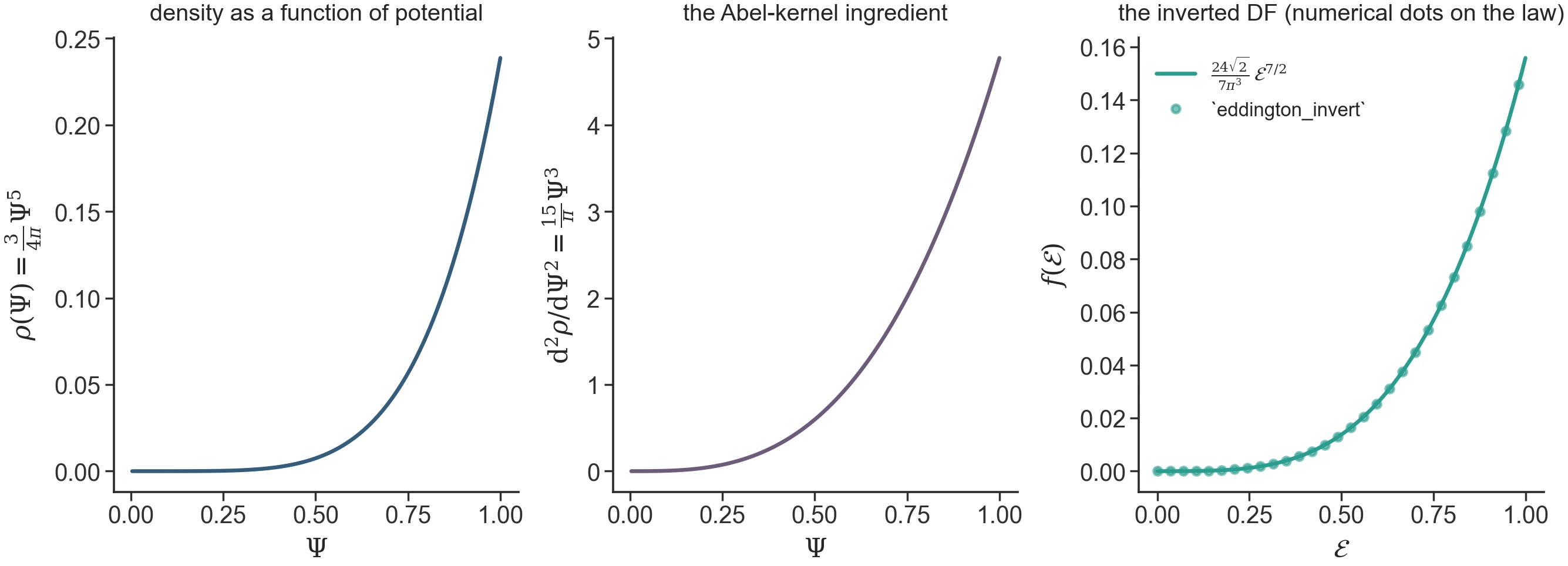
Figure 1:The inversion, step by step: the density as a function of the relative
potential, its second derivative (the Abel-kernel ingredient), and the
resulting DF — with the output of the numerical inverter
(eddington_invert, the same code Engine B uses) as dots on the closed-form
law. Max relative deviation with these grid inputs
( with analytic derivative inputs — the validation suite’s
strongest truth test). Regenerate: python -m laboratory.icviz --only eddington-triptych.
Closed-form moments¶
The first three velocity moments of the Plummer DF are
with . The ratio at all radii — this is the local statement of the virial theorem and the proximate reason a Plummer cluster sampled from (4) lands at at the DF level — realised as 0.5 up to the finite- Monte-Carlo fluctuation, with no rescale (What is an initial condition?).
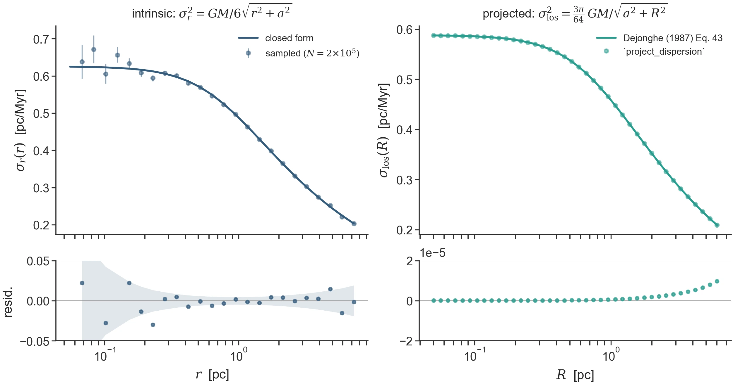
Figure 2:Both dispersion oracles, measured. Left: sampled
(, seed 11) threading the closed form, residuals inside the
Poisson band. Right: project_dispersion against the source-verified
Dejonghe (1987) Eq. 43 oracle — residuals (the
outer-radius rise is the documented master-interpolation floor).
Regenerate: python -m laboratory.icviz --only plummer-dispersion-oracles.
The central velocity dispersion is
which (combined with (3)) gives a one-line conversion between cluster mass, scale radius, and central velocity dispersion — useful for sanity-checking observational fits.
Sampling: speed and rejection¶
progenax samples velocities from (4) via inverse-CDF on the speed distribution at each particle’s position. At fixed , the DF integrated over angles gives
with . The distribution is bounded,
unimodal, and smooth, so progenax uses a fixed-iteration
inverse-CDF lookup table rather than rejection sampling. The lookup
table is constructed once per call (vectorised over ) and inverted
via jnp.interp, so the cost per particle is dominated by the
single bisection step — no Python loop, no rejection retries, fully
JIT-compatible.
Implementation in progenax¶
from progenax.kinematics import PlummerVelocityDF
from jaxstro.units import STELLAR
import jax, jax.numpy as jnp

df = PlummerVelocityDF(r_h=1.0)        # Half-mass radius in pc
masses = jnp.ones(1000)
key = jax.random.PRNGKey(42)
key_pos, key_vel = jax.random.split(key)   # never reuse a key

# Positions from the matched profile (any sampled positions work)
from progenax.profiles import PlummerProfile
positions = PlummerProfile(r_h=1.0).sample_positions(masses, key_pos)

# Sample velocities consistent with f(E) ∝ E^(7/2)
velocities = df.sample_velocities(positions, masses, key_vel, G=STELLAR.G)

# The DF is an exact equilibrium, so Q_vir -> 0.5 with no rescale
# (finite-N: 0.5 +/- ~5e-3 at N=1e4, the Monte-Carlo fluctuation)
PlummerVelocityDF is an Equinox module. Its single Python parameter
is r_h; everything else (the central potential depth, the inverse-CDF
lookup table) is derived analytically from inside the class.
Differentiability flows through .
Sanity checks¶
The Plummer DF satisfies four checks that progenax’s validation suite (Plummer equilibrium) verifies on every release:
Property | Tolerance | Source of truth |
|---|---|---|
Total kinetic energy / | Virial theorem (statistical from finite ) | |
Mean radial dispersion at | 1% of analytic value | |
Anisotropy parameter | Isotropy by construction | |
Bound fraction | All particles have for |
The first row implements the full Jeans-equation check: Plummer
positions sampled from PlummerProfile plus velocities from
PlummerVelocityDF produce to 0.5%, with
the residual being the finite- fluctuation of the Monte Carlo
energy estimate. No virial rescaling is needed — equilibrium is
exact at the DF level.
Check yourself¶
1. The 7/2 exponent by power counting
Without integrating: feeds the Abel kernel . Plummer has ; check that Dejonghe’s -family (which generalizes ) recovers the same at .
2. The central projected dispersion
Evaluate project_dispersion at and compare with
. With ,
(so pc, STELLAR units) you should get
pc/Myr — and it should agree with the
left panel’s central times … work
out that ratio () before running.
Anisotropy and rotation extensions¶
The Plummer DF above is isotropic () and non-rotating. progenax extends it with two compositions:
Osipkov-Merritt anisotropy: introduces a free anisotropy radius such that . The DF is no longer a function of alone but of , the augmented integral of motion. progenax implements this as an intrinsic DF option,
PlummerVelocityDF(r_h=..., anisotropy_radius=r_a), using the analytic OM Plummer DF (Merritt 1985, Eq. 45), which is non-negative only for (Merritt 1985, Eq. 46). See Anisotropy and rotation.Solid-body / differential rotation: adds a tangential velocity component to the isotropic Plummer velocities. Implemented via
apply_solid_body_rotation(df, omega)andapply_differential_rotation(df, omega_profile).
Both extensions are documented in detail at Anisotropy and rotation. They compose freely with each other and with non-Plummer profiles (e.g. King + Osipkov-Merritt is a common combination for old globular clusters with observed radial anisotropy).
Domain of validity and limitations¶
Single-mass equilibrium only. The Eddington DF assumes one stellar mass species. Multi-mass equilibrium DFs require simultaneous treatment of all mass groups — the multi-mass generalisation is formalized by Gieles & Zocchi (2015), which progenax plans to implement natively as its own differentiable generalization (see The differentiable lowered-model family (Engine A)).
Spherical and isotropic by default. Anisotropy and rotation extensions exist (above) but are layered on top of the isotropic DF; they do not change the underlying .
Untruncated. The DF extends to . For tidally truncated Plummer-like systems use King profile instead, or apply post-sampling truncation via
apply_tidal_truncation(Tidal physics).
Implementation, validation & references¶
In code:
src/progenax/kinematics/plummer_df.py(the isotropic , the inverse-CDF speed sampler, and the optional Osipkov–Merritt anisotropy) — see thePlummerVelocityDFAPI.Validated in: Plummer equilibrium — the regression suite that locks the velocity moments, isotropy , and the unscaled .
Primary sources: Plummer (1911) (the model and its DF); modern textbook treatments follow Binney & Tremaine Galactic Dynamics §4, and Aarseth et al. (1974) is a clean N-body initialisation reference — full notes in the bibliography. The mass-first sampling contract follows the IC redesign at IC redesign spec (2026-02-12).
- Plummer, H. C. (1911). On the problem of distribution in globular star clusters. Monthly Notices of the Royal Astronomical Society, 71, 460–470. 10.1093/mnras/71.5.460
- Dejonghe, H. (1987). A completely analytical family of anisotropic Plummer models. Monthly Notices of the Royal Astronomical Society, 224, 13–39. 10.1093/mnras/224.1.13
- Gieles, M., & Zocchi, A. (2015). A family of lowered isothermal models. Monthly Notices of the Royal Astronomical Society, 454, 576–592. 10.1093/mnras/stv1848
- Aarseth, S. J., Henon, M., & Wielen, R. (1974). A comparison of numerical methods for the study of star cluster dynamics. Astronomy and Astrophysics, 37, 183–187.