The stellar initial mass function (IMF) governs chemical enrichment, supernova rates, and the integrated light of galaxies. Measuring its shape — and whether it varies with environment — is one of the central problems in stellar astrophysics Salpeter, 1955Kroupa, 2001Chabrier, 2003Marks et al., 2012Jeřábková et al., 2018. Most stars do not form alone: roughly 50% of solar-type stars and >90% of O-type stars have at least one bound companion Sana et al., 2012Moe & Di Stefano, 2017. When those companions are unresolved, the IMF inferred from observed system masses is systematically biased toward shallower slopes.
This chapter is the single source of truth for the binary-aware IMF
recovery pipeline implemented in progenax.imf.BinaryIMF and exercised
in scripts/validate_binaries.py (fast MLE) and
validation/imf/validate_binary_aware_recovery.py (full numpyro NUTS). It derives the system mass
function under the Moe & Di Stefano (2017) joint binary statistics, formulates a
likelihood that marginalises over latent binary status and mass ratio, and
quantifies the regime — sample size — where the naive
single-star likelihood becomes “confidently wrong”: its 95% credible
interval shrinks below the bias and excludes the true slope.
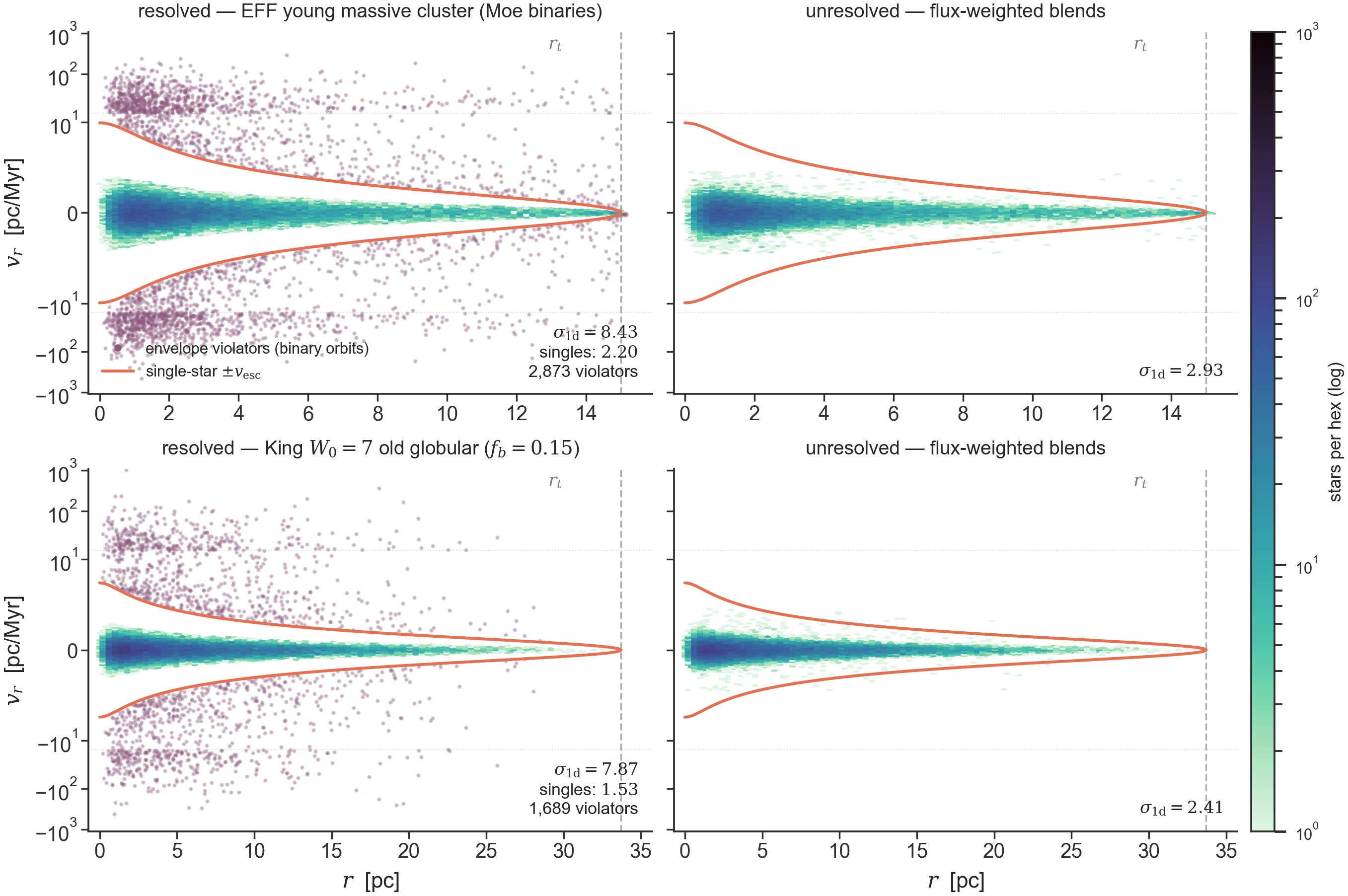
Figure 1:Binaries in phase space, and why they lie to your dispersion
(seed 21, systems each; symlog wings beyond
pc/Myr). Left column (resolved): plum points are
envelope violators — stars above the local single-star
that cannot be bound singles: 2,873 (EFF + Moe, top) and
1,689 (King + , bottom) contaminants reaching hundreds of
pc/Myr, inflating to 8.4 (singles: 2.2) and 7.9
(singles: 1.5). Right column (unresolved): each binary photometrically
blended (COM position, Tout-ZAMS flux-weighted velocity) — the violator
clouds all but vanish and the population looks clean, yet the measured
dispersion stays silently inflated (2.93 vs 2.20; 2.41 vs 1.53) — and the
few blend hexes still leaking past the envelope are near-equal-luminosity
pairs that keep half their orbital velocity. That hidden pedestal is exactly
the mechanism behind the binary-blind mass bias demonstrated on this page.
Regenerate: python -m laboratory.icviz --only binary-phase-space.
The Maschberger (2013) functional form
progenax uses the Maschberger (2013) “L3 distribution” as the single-star IMF backbone:
with default parameters (Salpeter high-mass slope), , . The high-mass limit recovers ; the second factor produces the observed turnover below
. Crucially, the cumulative distribution has a closed-form
inverse, enabling exact analytical sampling — no numerical root-finding,
fully jax.lax.scan-compatible, fully differentiable. See
`progenax.imf` for the implementation in
progenax.imf.Maschberger.
The binary contamination problem
For an unresolved binary system, the observer measures the system mass
where and is the mass-dependent binary fraction. Binaries transfer probability mass from intermediate to high system masses — a primary with appears as a single system. Consequently the observed system mass function is shallower than the true single-star IMF.
The naive practice of fitting a single-star IMF to the observed system masses — likelihood — converges as to the wrong value of . Kroupa (2001) quantified the bias at –0.10 depending on mass range and binary fraction. Section Paragraph below shows that the bias does not shrink with , and at LSST-scale samples (–105) the naive 95% credible interval becomes narrower than the bias and excludes the truth.
The Moe & Di Stefano (2017) joint binary statistics
Moe & Di Stefano (2017) compiled the most comprehensive census of binary star properties to date, combining spectroscopy, eclipsing binaries, long-baseline interferometry, adaptive optics, and common proper motion surveys. After correcting each sample for its selection function, they derived the intrinsic joint distribution of primary mass, mass ratio, orbital period, and eccentricity. Two findings shape progenax’s implementation:
Binary properties are not universal. Binary fraction, mass-ratio distribution, and period distribution all vary systematically with . Treating them as constants introduces correlated errors.
The joint distribution is not separable: . The mass-ratio distribution depends on both and ; eccentricity depends on ; companion frequency depends on both.
Binary fraction 
The mass-dependent binary fraction — the multiplicity fraction (, the probability of companion) — is tabulated, with its full per-mass values and provenance (Moe & Di Stefano (2017) Table 13 single-star row for , M-dwarf surveys below), in the canonical multiplicity-statistics chapter. The trend is steep: O-type stars are almost always in multiples (), while M-dwarfs are mostly single (–0.3) — a factor-of-4 dynamic range that is the leading-order driver of the binary-IMF bias.
This is the multiplicity fraction, not the companion frequency , which exceeds 1.0 ( per O-type primary, Moe & Di Stefano (2017) Table 13) once hierarchical triples are counted — see Limitations below for the single-companion approximation progenax adopts.
Mass-ratio distribution 
For a primary of mass , Moe & Di Stefano (2017) parameterise as a power law plus a narrow “twin excess” peak near :
where and . progenax uses a period-averaged single-slope — a reduction of Moe & Di Stefano (2017) Table 13’s period-dependent (averaged over ) — appropriate for total mass-function analyses, but losing the small- structure that matters for surveys sensitive to specific period ranges (see Limitations). The per-mass and tables live in the canonical Mass-ratio distributions.
Qualitatively, the slope trend reverses at high masses: massive stars preferentially have low-q companions (), while low-mass stars prefer near-equal-mass companions (). The twin fraction peaks at solar-type primaries ( for 0.8–) and falls to 0.03 for .
The system mass function
Given the forward generative model — draw from the IMF, decide binary or not, add if binary — the probability density of the observed system mass is
The binary term integrates over every primary mass that could produce the observed system mass , weighted by the IMF, the binary fraction, and the mass-ratio distribution. The integration limits come from : implies ; implies . The Jacobian arises from the change of variables .
This integral has no closed form because and are piecewise functions of . progenax evaluates it via 128-point Gauss-Legendre quadrature, which gives ~14 digits of accuracy for smooth integrands.
The binary-aware likelihood
For an observed system mass :
where is evaluated at the candidate primary mass inside the integral. The integrand is smooth in , so Gauss-Legendre quadrature on converges fast.
Computational cost. For observed systems and 128 quadrature points,
each likelihood evaluation requires IMF + mass-ratio
evaluations. At (LSST-scale) this is
evaluations per NUTS step, flops per chain. On a
MacBook Pro CPU one chain takes minutes; on an A100 the same
tile is embarrassingly parallel via jax.vmap, bringing
the per-chain time down to s — an estimated
speedup (see Binary-aware likelihood for the per-step breakdown).
Confidently wrong: the naive likelihood at large N
The naive likelihood is a misspecified model: the data-generating process includes binaries; the likelihood does not. As both naive and binary-aware posteriors shrink as (Bernstein–von Mises), but they shrink around different values:
The binary-aware posterior shrinks around .
The naive posterior shrinks around , where –0.10 is set by the binary statistics and is independent of .
The 95% credible interval shrinks; the bias does not. At some the CI becomes narrower than the bias, and the posterior excludes the true value:
progenax binary-aware validation results, Salpeter .
Naive 95% CI width | Naive | Status | |
|---|---|---|---|
500 | 0.28 | 0.045 | CI contains truth |
1{,}000 | 0.20 | 0.035 | CI contains truth |
3{,}000 | 0.12 | 0.057 | CI contains truth (barely) |
10{,}000 | 0.06 | 0.082 | CI excludes truth |
30{,}000 | 0.035 | 0.098 | Confidently wrong |
This regime — narrow posterior centred on the wrong answer — is the central danger of ignoring binaries with large datasets. progenax’s binary-aware likelihood eliminates the bias by construction; the cost of the inner -quadrature is the price.
Observation operators: what does the telescope measure?
The likelihood (5) uses the dynamical-mass operator . This is exact for eclipsing binaries, SB2 spectroscopic binaries, and astrometric binaries — observations that recover the true system mass. It overstates the distortion for photometric surveys, where the telescope measures combined flux rather than combined mass.
For a main-sequence luminosity scaling with –4, the inferred photometric mass of an unresolved binary is
Because , the secondary contributes appreciably to the flux only when :
Photometric vs. dynamical mass for .
() | Comment | ||
|---|---|---|---|
1.0 | 0.75 mag brighter | ||
0.5 | Companion barely changes flux | ||
0.3 | Negligible photometric effect |
The mass-addition operator therefore gives an upper bound on the binary distortion. Photometric masses are much less affected, especially at moderate — but the bias does not vanish, and the naive model still becomes confidently wrong at sufficiently large . Full LSST-realistic inference replaces with isochrone-mediated flux addition; see the Add a binary population recipe for the planned extension.
Limitations
Implementation in progenax
The pipeline lives in three modules:
progenax.imf.BinaryIMF— the Moe & Di Stefano (2017)-conditioned forward model and likelihood. Differentiable viajax.grad, JIT-compatible, vectorisable viajax.vmap.progenax.binaries.MoeEccentricityand friends — the joint binary statistics tables used byBinaryIMF(see Binary period distributions).scripts/validate_binaries.py— the fast (MLE, no-MCMC) figure suite that regenerates the “ vs. CI vs. bias” result;validation/imf/validate_binary_aware_recovery.pyis the full numpyro NUTS cross-check.
See `progenax.imf` for full API signatures and Add a binary population for a recipe building a binary-corrected mock catalog end-to-end.
Implementation, validation & references
In code:
src/progenax/imf/binary/imf.py(BinaryIMF— the forward model and sampling helpers), with the joint statistics insrc/progenax/imf/binary/moe_di_stefano.pyand the single-star backbone insrc/progenax/imf/smooth.py(Maschberger) — see the IMF API. The recovery figures are regenerated byscripts/validate_binaries.py(fast MLE) andvalidation/imf/validate_binary_aware_recovery.py(full numpyro NUTS).Validated in: binary-aware recovery — the regression suite that demonstrates unbiased recovery at where the naive fit is confidently wrong.
Primary sources: the single-star backbone is Maschberger (2013); the binary-contamination statistics are Sana et al. (2012)Moe & Di Stefano (2017)Moe et al. (2019); the “confidently wrong” framing is original to progenax. Full notes in the bibliography. For the environment-dependent IMF that consumes from this chapter, see Environment-dependent IMFs.
- Salpeter, E. E. (1955). The luminosity function and stellar evolution. The Astrophysical Journal, 121, 161–167. 10.1086/145971
- Kroupa, P. (2001). On the variation of the initial mass function. Monthly Notices of the Royal Astronomical Society, 322, 231–246. 10.1046/j.1365-8711.2001.04022.x
- Chabrier, G. (2003). Galactic stellar and substellar initial mass function. Publications of the Astronomical Society of the Pacific, 115, 763–795. 10.1086/376392
- Marks, M., Kroupa, P., Dabringhausen, J., & Pawlowski, M. S. (2012). Evidence for top-heavy stellar initial mass functions with increasing density and decreasing metallicity. Monthly Notices of the Royal Astronomical Society, 422, 2246–2254. 10.1111/j.1365-2966.2012.20767.x
- Jeřábková, T., Kroupa, P., Dabringhausen, J., Hilker, M., & Bekki, K. (2018). Impact of metallicity and star formation rate on the time-dependent, galaxy-wide stellar initial mass function. Astronomy and Astrophysics, 620, A39. 10.1051/0004-6361/201833055
- Sana, H., de Mink, S. E., de Koter, A., Langer, N., Evans, C. J., Gieles, M., Gosset, E., Izzard, R. G., Le Bouquin, J.-B., & Schneider, F. R. N. (2012). Binary interaction dominates the evolution of massive stars. Science, 337, 444–446. 10.1126/science.1223344
- Moe, M., & Di Stefano, R. (2017). Mind your Ps and Qs: The interrelation between period (P) and mass-ratio (Q) distributions of binary stars. The Astrophysical Journal Supplement Series, 230, 15. 10.3847/1538-4365/aa6fb6
- Maschberger, T. (2013). On the function describing the stellar initial mass function. Monthly Notices of the Royal Astronomical Society, 429, 1725–1733. 10.1093/mnras/sts479
- Moe, M., Kratter, K. M., & Badenes, C. (2019). The close binary fraction of solar-type stars is strongly anticorrelated with metallicity. The Astrophysical Journal, 875, 61. 10.3847/1538-4357/ab0d88