When a source parameter shifts, a derivative names what changes in the observable and under which assumptions. It is a local rate of change, the best local linear map approximating a function, and a scientific sensitivity. The object and the perturbation come first; AD supplies a way to evaluate the chosen derivative.
View 1: local change
For a scalar function, the derivative at is the limiting ratio
This says more than “slope on a graph.” It names which input changes, which output changes, their units, and the local point. For Newtonian gravity, derivatives with respect to mass and separation answer different scientific questions. For Stefan-Boltzmann luminosity, temperature sensitivity carries luminosity-per-temperature units.
View 2: the best local linear map
Near , a differentiable function satisfies
is a linear map from input perturbations to output perturbations. In coordinates it becomes a derivative, gradient, or Jacobian depending on shapes and conventions. A directional derivative applies the map to one direction. This formulation scales from one variable to millions.
A JVP computes : push one input perturbation forward. A VJP computes : pull one output sensitivity backward. Reverse-mode gradients are VJPs of a scalar output, not a magical new type of derivative. Tangent vectors carry input perturbations; cotangent vectors carry linear measurements of output perturbations.
View 3: scientific sensitivity and evidence
A derivative always belongs to a mapping. In statistics, the gradient of a log likelihood is the likelihood score. A Hessian records local curvature. Fisher information summarizes expected score geometry under a specified probabilistic model. None of these is meaningful without the model, parameterization, data distribution, and point of evaluation.
For a root defined by , an implicit sensitivity can be derived on a unique smooth branch:
This derivative becomes unstable when the denominator is poorly conditioned and is not justified when uniqueness or smoothness fails.
The derivative of a relation versus an executed program
JAX differentiates the represented map according to primitive and custom
transformation rules. Ordinary pathwise AD follows selected branches, finite
iteration counts, clamps, and represented arithmetic. But custom_jvp,
custom_vjp, and custom_root deliberately install derivative semantics that
need not differentiate the executed primal iteration history. Jaxstro’s
certified implicit API uses the latter pattern. It therefore distinguishes
smooth finite-map derivatives, value-first iterative maps, validation-only
finite-difference checks, and separately defined implicit derivatives.
At a branch boundary, knot, absolute-value kink, clipping threshold, repeated root, or discrete selection, a classical derivative can fail to exist or become branch-dependent. A finite number returned by AD does not settle that question.
Why this motivates differentiable programming
Differentiable programming makes local linear maps composable across a program. The same machinery supports physical sensitivity analysis, inverse problems, uncertainty propagation, optimization, control, experimental design, and probabilistic inference. Its power comes from composition; its scientific validity still comes from model and derivative contracts.
Try the running case
In the two-channel measurement, a parameter vector predicts the data. At a reference point, decide whether the question is about the change in predicted measurements under a proposed , or about the change in a scalar loss after those measurements are compared with data.
Worked audit
The first question is a JVP, , and retains the direction and units of the predicted measurement change. The second is a VJP after a scalar objective has supplied an output cotangent. They can share implementation machinery, but they answer different scientific questions and should not be reported as the same sensitivity.
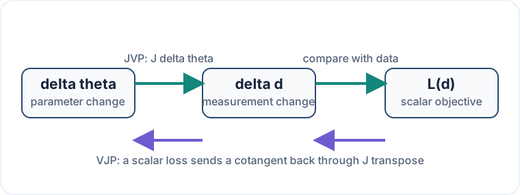
Figure 1:A JVP carries a proposed physical change forward. A VJP carries the chosen measurement or loss sensitivity back. They share a map and differ in the question asked of it.
Name the input, output, evaluation point, units, held-fixed quantities, desired derivative meaning, smooth branch, and expected sign before invoking AD.
Choose forward or reverse products from input/output geometry. Retain solver certificates and control-flow information; make a nonsmooth selection visible in the derivative contract.
Compare with an analytic derivative, central finite differences at several step sizes, complex-step where admissible, or an independent implicit calculation. Probe both sides of suspected boundaries and monitor conditioning.
Continue to Sensitivity, conditioning, and identifiability, From mathematical relations to differentiable programs, or Jaxstro’s Autodiff products and Root-finding chapters.