A stellar luminosity, a gravitational force, and a detector count become useful only after their inputs, outputs, units, and allowed limits are fixed. The same algebraic expression can answer different questions when any one of those choices changes.
A function carries physical commitments
Newtonian gravity gives the scalar force magnitude,
The relation excludes zero separation. Its output has force units; doubling a mass doubles the force, while increasing separation weakens it as . A vector force also needs a direction convention. A scalar magnitude with the wrong direction does not describe the force.
The Stefan-Boltzmann relation
maps stellar radius and effective temperature to bolometric luminosity under specific physical assumptions. Near a chosen state, a fractional change in temperature has four times the fractional effect of the same change in radius. The relation does not supply an atmosphere model or a band-limited flux.
The same relation can use SI, CGS, or solar scales
The physical relation stays fixed while its numerical representation changes. For gravity, the coefficient must match the mass, length, and time inputs:
The factor of 103 reflects the conversion of cubic length and mass together;
it is not a change in the force law. Jaxstro’s foundation uses CGS by default,
so G_CGS expects grams, centimeters, and seconds unless a caller supplies a
different explicit unit system or constant.
Stellar work often benefits from a third representation. Jaxstro records the IAU nominal conversions
Thus a luminosity of is the same physical power as
or .
The solar radius and luminosity are nominal conversion factors, not measurements
of a changing Sun. MSUN_G is different: it is Jaxstro’s documented rounded
compatibility scale, not an IAU nominal solar mass. That distinction matters
when a calculation needs an absolute mass convention rather than a convenient
stellar-scale coordinate.
| Scientific setting | Useful explicit basis | What stays invariant |
|---|---|---|
| Laboratory or instrument calibration | SI: kg, m, s, W | The dimensional relation and the measured observable |
| Stellar structure or luminosity | CGS internally; and at a reporting boundary | The physical radius and power |
| Binary or planetary orbit | , AU, yr | The orbit; is a convenient numerical representation |
Units reject incompatible operations, expose missing scale factors, and keep a coordinate distinct from a dimensionless ratio. A dimensionless angle, relative residual, and probability carry different semantics even though each has no base units.
Scaling makes the numerical coordinate explicit
Writing a physical quantity as separates a reference scale from the dimensionless numerical coordinate . For a stellar luminosity, makes easy to read without hiding the conversion back to watts or erg s. For a numerical kernel, choose before tracing or compiling; pass the dimensionless values through the kernel and restore units at the boundary. This can reduce scale-driven conditioning problems. An order of magnitude estimate of each term should choose the scale before a solver or an accelerator sees the calculation. Scaling cannot fix a bad model, cancellation from an unstable formula, or an unidentified parameter direction.
Try the running case
In the two-channel measurement, let a physical prediction have watts. The first instrument records in watts; the second records in detector counts for a calibration factor in counts per watt. Before fitting , write the units of , , , and . Which two quantities may be subtracted without a conversion?
Worked audit
and have the same units, so is meaningful. The residual mixes counts and watts. Compare in counts, or convert to watts while carrying the calibration uncertainty. Scaling numerical values near one can help a solver; it cannot make the residual dimensionally valid.
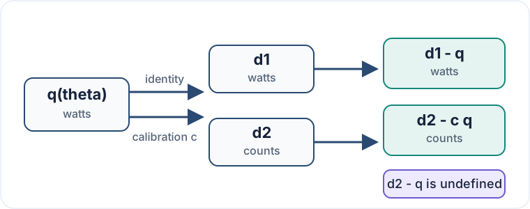
Figure 1:The calibration changes the numerical representation of the same predicted signal. It does not authorize a residual that mixes counts with watts.
For the chosen gravity, luminosity, or detector relation, record the expected units, sign, monotonic direction, limiting behavior, and dominant scale before evaluating it.
Choose SI, CGS, or a named astrophysical basis explicitly. Convert once at a visible boundary, retain named physical variables, and keep nondimensional kernel coordinates separate from the quantities they represent.
Check dimensions, an analytic ratio, a limiting case, and an independent evaluation. For tabulated or iterative code, inspect coverage and status as well as the returned value.
Continue to What is a model? or the numerical Quantities, units, and dimensional boundaries module page.