Probability and distributions

Recorded measurements vary for reasons that belong to the experiment, the instrument, and the model. Probability states which variations the analysis admits; it does not identify their physical origin by itself.

Mass, density, and support¶

For discrete outcomes, probability mass assigns probabilities that sum to one. For continuous quantities, a probability density integrates to one but is not itself the probability of an exact point. Density carries reciprocal units of its variable. The support states which outcomes the model admits; behavior outside support is part of the contract.

Normalization makes the total probability one. In a finite stellar-mass power law, the normalization changes smoothly with the exponent and has a logarithmic removable limit. A correct formula must preserve values and parameter derivatives through that limit.

For a continuous variable on support $\mathcal{X}$ , normalization and an expectation are explicit operations:

\int_{\mathcal{X}} p(x)\,dx = 1, \qquad \mathbb{E}[g(X)] = \int_{\mathcal{X}} g(x)p(x)\,dx.

(1)

Summaries and dependence¶

An expectation is a probability-weighted average under a specified distribution. Variance measures squared spread about an expectation. Covariance records linear co-variation and has product units; correlation is its dimensionless normalized form. These summaries do not uniquely determine a general distribution.

Conditioning, written $p(x\mid y)$ , changes the distribution of one quantity given information about another. It is not the same as numerical conditioning, though both concepts appear in scientific inference.

Transformations and sampling¶

A transformation changes density through its local volume factor, not merely by substituting values. Sampling produces draws from a specified distribution; it does not validate that distribution as a model of nature. Inverse-CDF sampling depends on normalization, monotonicity, support, and a reliable quantile map.

Kinds of uncertainty¶

Aleatoric uncertainty represents variation modeled as intrinsic to the data- generating process. Epistemic uncertainty represents limited knowledge about models, parameters, or missing structure. The boundary is model-dependent: a latent physical variable treated as noise in one analysis may become explicit state in another.

Try the running case¶

The two-channel measurement is collected in a data vector $d$ . Suppose its reported errors are centered and have covariance $C$ . Before calling either error “Gaussian,” ask which data values the model admits, whether the measurements can co-vary, and what mechanism could make their errors share a calibration offset.

Worked audit¶

A Gaussian likelihood is a model choice, not a synonym for an error bar. If the two calibrated measurements share a calibration offset, the off-diagonal entries of $C$ need not vanish. A support restriction or a heavy-tailed error model changes the likelihood even if the reported standard deviations are the same. The next page makes the forward and measurement maps explicit.

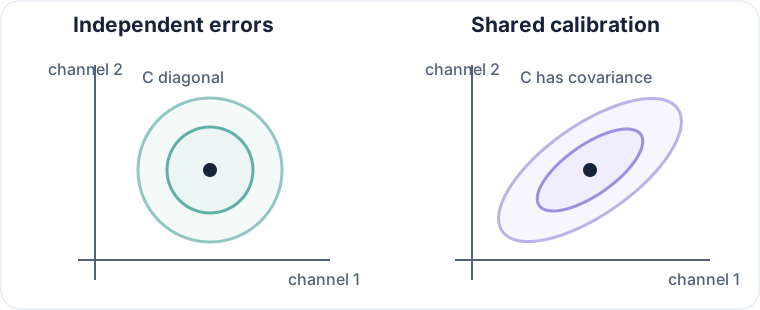
Independent error contours are circular in two-channel data space, while a shared calibration uncertainty creates tilted contours through the same observed point. — Figure 1:The tilted cloud encodes a specific measurement mechanism: both channels move together when the calibration moves. Reporting two separate error bars loses that information.

Predict

Name the random variable, support, units, normalization, expected symmetries, limiting cases, and the uncertainty represented.

Compute

Evaluate density, CDF, quantile, moments, or samples with explicit boundary behavior. Use stable limiting kernels and keep random seeds and transformations in the evidence record.

Audit

Check normalization, nonnegativity, support boundaries, monotonic CDF behavior, CDF/quantile round trips, analytic moments where available, and parameter derivatives against an independent method.

Continue to Models, inference, and information or Jaxstro’s Distribution kernels chapter.