When two source parameters change the same measurements, three different questions arise: how strongly the observable responds, whether arithmetic can resolve that response, and whether the experiment separates the parameters.
Sensitivity
Sensitivity describes how an output changes under a specified input perturbation. It can be local or global, dimensional or normalized, and tied to a physical parameter, initial state, observation, or numerical control. A large derivative may be physically expected rather than numerically problematic.
For a local observable map, the first-order response is
When a covariance is an appropriate positive-definite measurement-error model, the local information geometry is often summarized by
This Fisher form is conditional on the local linearization and covariance assumptions; it is not a proof of global identifiability.
Conditioning
Conditioning describes how perturbations in inputs or arithmetic can be amplified by a problem. It belongs to the problem and representation; stability describes how an algorithm handles that problem. Parallax inversion becomes poorly conditioned as parallax approaches zero. A root sensitivity becomes poorly conditioned when the residual slope approaches zero.
Scaling can improve numerical representation. It cannot remove physical degeneracy, and a sophisticated solver cannot make an ill-conditioned question well-conditioned.
Identifiability and degeneracy
Identifiability asks whether different parameter values imply distinguishable predictions under a model and experiment. A degeneracy is a direction or manifold along which predictions change little or not at all. Locally, a Jacobian null space contains a null direction invisible to first order.
Identifiability may be structural, practical, local, or global. A full-rank local Jacobian does not exclude distant alternative solutions. A prior can select among weakly identified values without changing the likelihood information.
Derivative evidence
Automatic differentiation computes derivatives of represented programs accurately up to floating arithmetic, but it does not decide whether the intended mathematical derivative exists. Finite differences supply an independent discretization with truncation and cancellation error. Agreement across a stable step range is evidence; disagreement is a diagnostic, not a reason to choose the more convenient answer.
Use analytic derivatives, JVPs/VJPs, central differences, convergence, singular values, and model perturbations as complementary evidence. The correct audit depends on branch smoothness and the scientific question.
Try the running case
For the two-channel measurement with two source parameters, if the Jacobian columns are nearly parallel, decide which statement follows: the code has a bug, the numerical representation is poorly scaled, or the measurements weakly distinguish one parameter combination.
Worked audit
Near-parallel columns establish a local weak direction of the stated observable map. They do not by themselves diagnose a code bug or forbid a stable forward calculation. Rescaling can improve arithmetic; an additional observable or a justified prior can change the inference. Those are different interventions and must be evaluated against the scientific question.
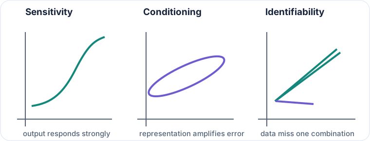
Figure 1:Large response, poor conditioning, and weak identifiability can coexist, but none implies either of the others. The remedy follows the diagnosis.
Predict sensitive directions, expected signs and units, possible degeneracies, boundary behavior, and conclusions that should change under rescaling or model perturbation.
Evaluate local derivatives and normalized sensitivities; inspect Jacobian or Fisher singular directions; record numerical tolerances, parameterization, and the experiment defining the observable map.
Compare AD with analytic or finite-difference results away from nonsmooth boundaries. Change scaling and parameterization, probe global alternatives, and test whether added observations constrain the predicted null directions.
Continue to From mathematical relations to differentiable programs.