The question this method answers
Given a scalar relation , what value of satisfies it, and which derivative of that answer is scientifically meaningful? A robust root value, the sensitivity of a finite executed solver, and the sensitivity of a unique smooth mathematical root are different objects.
The derivative distinction begins in What is a derivative?. Parameter and state representations are connected in Parameters, constraints, and transforms.
Before computation: what should be true?
Define the scalar variable, residual units, parameters, expected root branch, and admissible interval. For a sign-bracketed solve, must be continuous on the interval and its endpoints must have opposite signs or contain an exact root. For an implicit derivative, the selected root must also be unique and smooth in the parameter, with a finite nonzero local slope .
Pick tolerances in root-coordinate units. atol has the units of and
rtol is dimensionless. Enable sufficient precision before requesting a
tolerance near float64 limits.
Define the mathematical objects
A root is such that . A bracket at iteration is an ordered interval with evaluated endpoint residuals. The best endpoint is the one with smaller absolute residual. A proposal is a candidate inside the bracket, produced by bisection, secant interpolation, or inverse-quadratic interpolation (IQI).
A fixed trace stores the proposal, its residual, updated endpoint evidence, proposal kind, execution mask, admissibility, convergence state, and terminal status for every allocated scan slot. Unused floating entries are NaN and unused mask entries are false; fixed shape is an execution contract, not a convergence claim.
For a parameterized root relation, define and on the selected smooth branch. These local derivatives belong to the mathematical relation, not to the branch history of a numerical solver.
Derive the method
Bracket preservation and bisection
A verified bracket preserves the opposite-sign endpoint invariant
Sign bits or exact endpoint zeros are safer in floating point than multiplying large or tiny residuals. Bisection evaluates and replaces the endpoint that has the same sign as . Therefore . After steps,
This is a value-error certificate for a continuous sign-changing residual; it does not create a useful derivative with respect to parameters inside .
Safeguarded interpolation
Secant interpolation uses the line through the endpoint pairs. IQI fits the inverse relation through three distinct residual points. The current proposal code tries inverse-quadratic interpolation when three distinct residual points exist; otherwise the endpoint secant is selected. The selected interpolant must be finite, strictly inside the bracket, make sufficient progress, and stay inside the safeguard band
The safeguard band is inclusive; a proposal on either band edge is admissible when it also satisfies the separate finite, strict-interior, and progress checks. A rejected selected interpolant falls back to the overflow-safe midpoint. The bracket update then restores (1).
Newton and the implicit derivative
Newton linearizes the residual about : . Setting the approximation to zero gives
For a unique smooth mathematical root, differentiate :
This implicit function theorem (IFT) result requires a nonzero denominator and the stated uniqueness and smooth-branch assumptions. It is not obtained by differentiating bisection decisions.
Inverse CDFs
For a cumulative distribution , the quantile solves and . Newton therefore becomes
This finite inverse-CDF construction is not a generic implicit-root certificate.
What the algorithm actually does
bracket_expand(f, x0, step=1, growth=2, max_steps=32) searches symmetric
intervals with a fixed scan and returns (lo, hi, found). If discovery fails,
the returned endpoints are the last expanded interval and found=False.
bisect(..., max_steps=50) performs a caller-selected fixed number of
halvings, with default max_steps=50; bisect_many is the explicit
array-shaped wrapper for independent brackets.
initialize_bracket constructs true endpoint evidence from already evaluated
residuals. update_bracket(..., valid=False) leaves every field unchanged.
BracketedRootState pairs BracketState with interpolation-only
BracketHistory; propose_bracketed proposes without evaluating, and
advance_bracketed_root consumes one externally supplied evaluation.
Proposal-kind telemetry
Identifier | Value | Meaning |
|---|---|---|
|
| Masked slot or missing bracket |
|
| Endpoint secant accepted |
|
| Selected interpolant rejected; deterministic midpoint used |
|
| Exact lower-endpoint root |
|
| Exact upper-endpoint root |
|
| Three-point IQI accepted |
safeguarded_bracketed_root evaluates both endpoints and runs max_steps
fixed lax.scan slots. A scalar lax.cond prevents residual evaluation after
convergence or terminal failure. Convergence is an exact residual or a full
bracket width no larger than
. Exhaustion returns the
evaluated endpoint with smaller absolute residual and converged=False.
A missing bracket returns NaN root and residual with bracketed=False; a
nonfinite interior evaluation terminates that lane.
RootTrace and BracketedRootResult retain the fixed trace, status, final
bracket, initial residual scale, and function-evaluation count. The no-extra-
evaluation guarantee is scalar. vmap preserves values and shapes but can
lower lax.cond to select-style execution; map_safeguarded_bracketed_root
owns an explicit lax.map boundary when physical per-lane skipping matters.
What JAX differentiates
bisect, bracket discovery, and safeguarded proposals select intervals through
sign and acceptance predicates. Their parameter gradients are branch-selected
finite-program artifacts, not root sensitivities; bisection is structurally
zero with respect to parameters captured only inside .
newton and newton_with_grad use smooth iterates, finite-map gradients.
Their caller-selected fixed update count has default max_steps=30. JAX can
expose a finite executed-map sensitivity through those updates, but that is not
automatically (5). The zero-derivative operand is
replaced by one before division to avoid dead-branch poisoning; this guard
preserves finiteness, not convergence.
implicit_bracketed_root(f, args, ...) is separate. It uses lax.custom_root
and exposes a certified mathematical-root sensitivity only after caller
assertions of uniqueness and a smooth branch plus convergence, finiteness,
residual, bracket-width, and slope-conditioning gates. Rejection returns NaN
for the derivative-facing value and attempted gradient while retaining the
nested primal diagnostics.
newton_ppf adds pdf_floor to its denominator and clips every iterate to
[lo, hi]. Interior iterates can carry finite executed-map sensitivity with
respect to and parameters in the CDF. At a clipped support boundary the
gradient saturates to zero. monotone_inverse_interp is linear inside table
cells and clamps outside the tabulated range.
Using it in Jaxstro
Use the actual owner path and inspect the typed result rather than extracting a number without its status:
from jaxstro.jaxconfig import enable_high_precision

enable_high_precision()  # before creating JAX arrays

from jaxstro.numerics.rootfinding import safeguarded_bracketed_root


result = safeguarded_bracketed_root(
    lambda x: x**2 - 2.0,
    0.0,
    2.0,
    max_steps=64,
    atol=1.0e-12,
    rtol=1.0e-12,
    safeguard_fraction=0.1,
)
assert result.bracketed
assert result.converged
The safeguarded interface is scalar and returns fixed-length trace arrays.
Batched callers map scalar solves explicitly. The function and iteration count
are static when wrapped in jax.jit.
Table 2:Choosing a one-dimensional solver
Need | Use | Derivative meaning |
|---|---|---|
Discover a sign change |
| Value evidence only |
Simple robust bracketed value |
| No parameter-root derivative claim |
Auditable expensive bracketed value |
| Value-first branch-selected map |
Downstream-owned trial evaluation | bracket primitives | Value-first checkpoint surface |
Smooth residual and good guess |
| Finite executed-map sensitivity |
Unique smooth certified root |
| Certified mathematical-root sensitivity |
Smooth inverse CDF |
| Finite executed-map sensitivity |
Monotone inverse table |
| Cell-local query sensitivity |
How to audit the result
Predict -> compute -> audit: which derivative are you asking for?
Predict. State whether the target is a root value, the finite executed algorithm, or a unique smooth mathematical root. Derive the expected sensitivity.
Compute. Retain signed endpoint residuals, trace, status, final bracket, local slope, and every certificate predicate.
Audit. Check the opposite-sign endpoint invariant is checked at every executed update. Compare the certified AD derivative with the analytic result and an independently recomputed central finite difference. Reject the claim if uniqueness, smoothness, residual, width, finiteness, or conditioning fails.
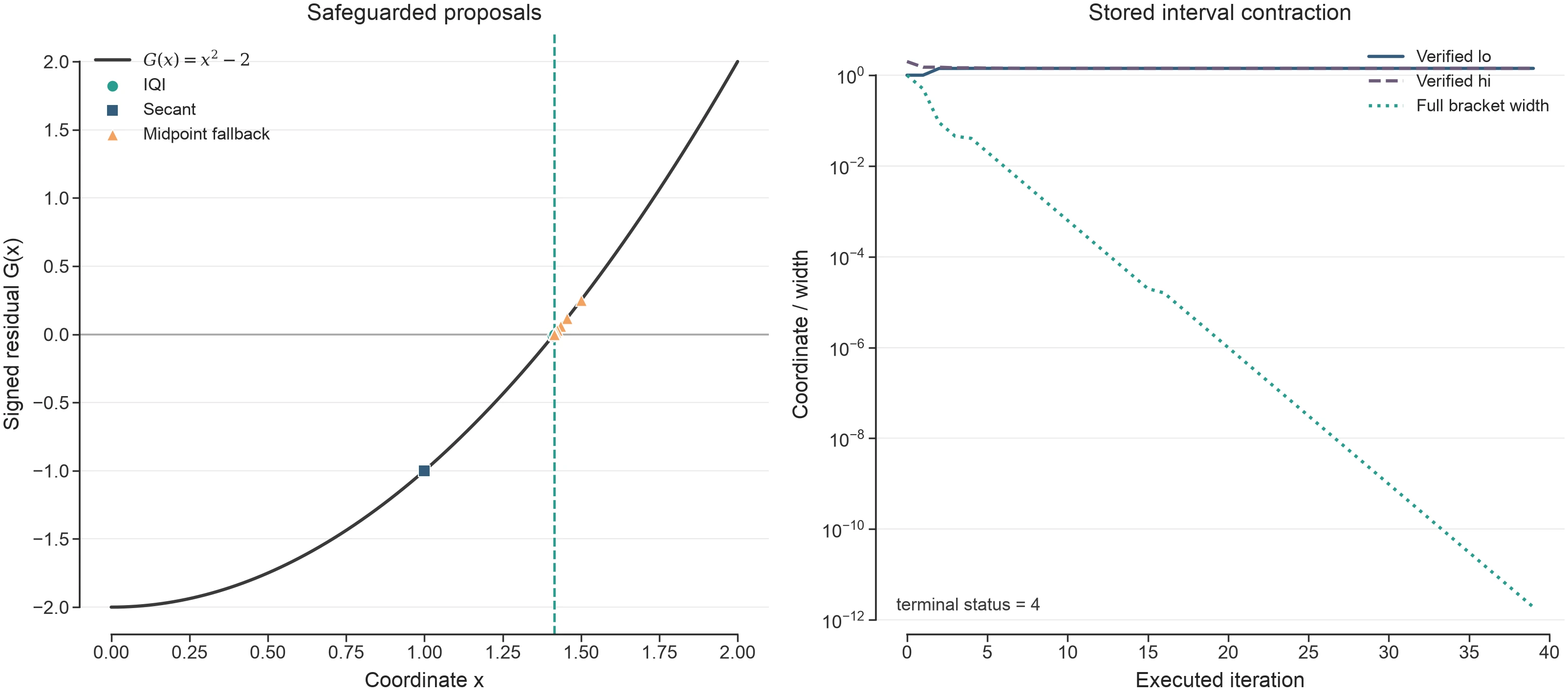
Figure 1:The public trace supplies every plotted point. The figure demonstrates interval telemetry and the opposite-sign endpoint invariant; it does not claim universal speed.
The reproducible evaluation-count report is
rootfinding
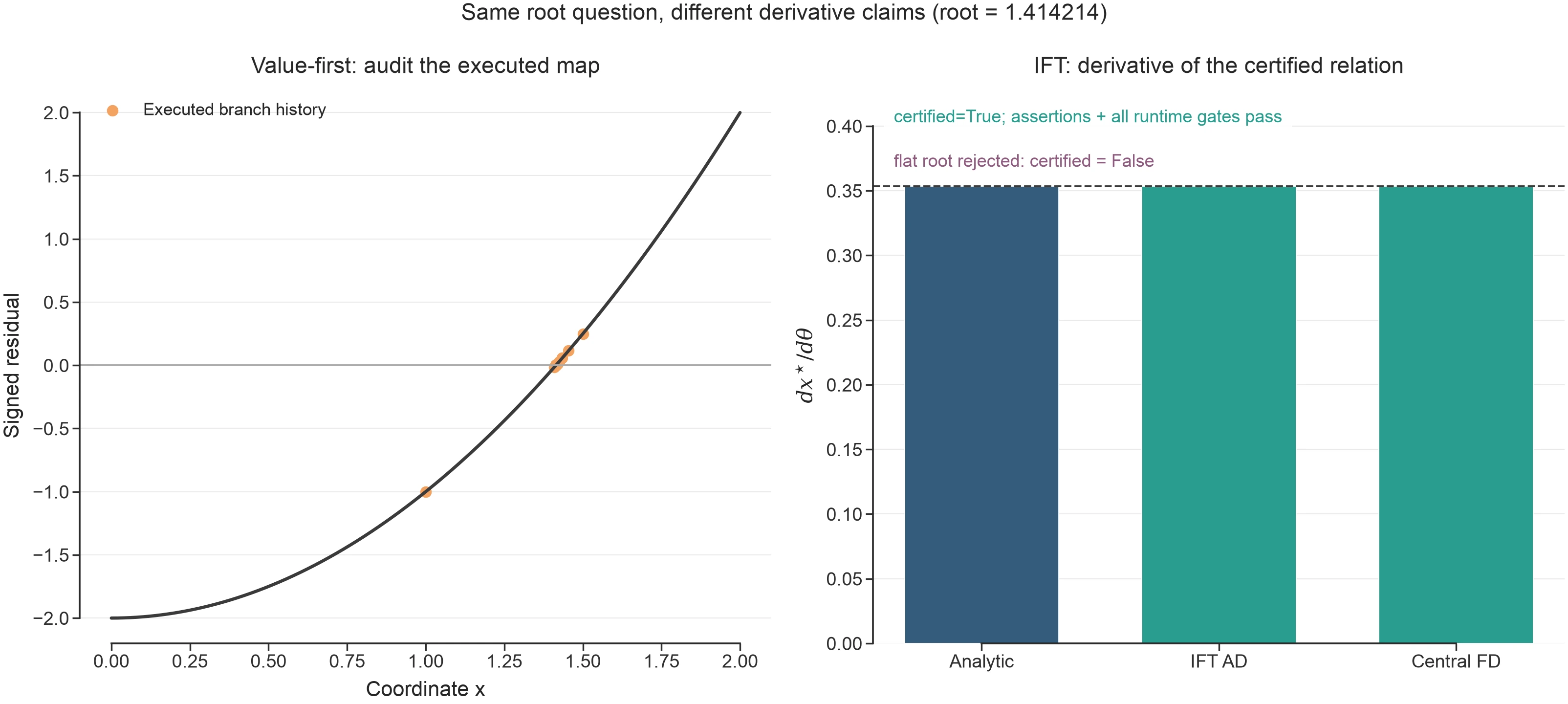
Figure 2:The left panel asks what numerical map executed. The right asks how the certified root relation moves with its parameter. The flat-root case is a rejection, not an estimate.
Figure 2 keeps the executed-map and certified-root derivative questions visually separate.
Measured quadratic implicit-root evidence
Metric identity | Symbol | Value | Units |
|---|---|---|---|
Certified root |
| coordinate units | |
Final absolute residual |
| function units | |
Final bracket width |
| coordinate units | |
Implicit-function AD sensitivity |
| coordinate units per parameter unit | |
Central-FD root sensitivity |
| coordinate units per parameter unit |
The machine-readable envelope and human report are generated and freshness-
checked together; see rootfinding
Where the claim stops
A valid bracket does not prove uniqueness. A small residual alone can hide an ill-conditioned root. A narrow bracket certifies coordinate location only under the continuity and sign-change assumptions. Successful JIT or VMAP execution does not add derivative meaning, and a warm benchmark does not establish performance for a different residual cost or batch structure.
The exponential inverse-CDF check validates one smooth interior case. It does not certify all distributions, clipped quantiles, traced invalid tables, or model-specific branch semantics.