Two source parameters can move two measured channels at the same time. Treat vectors as perturbations, then ask which combinations the data see, which they miss, and how numerical coordinates alter that diagnosis. A matrix is a coordinate representation of the map after choosing a basis; the map and its visible directions are the scientific objects.
Vectors, coordinates, and linear maps
A vector can represent a position, but it can also represent a small change in model parameters, a residual spectrum, a velocity, or a direction through parameter space. A map is linear when it preserves addition and scaling:
A basis supplies coordinates for a vector. In a basis whose vectors are the columns of , the same abstract vector has coordinates through
Changing basis changes coordinates and the matrix representing a map, not the underlying vector or map. Units and scaling remain part of the scientific meaning of those coordinates: a parameter measured in kelvin and one measured in dex should not be treated as interchangeable numerical axes simply because both appear in one array.
Geometry: dot products, norms, and projection
The Euclidean dot product and norm are
They define the angle through
If the columns of are an orthonormal basis for a subspace , its Euclidean projection is
This geometry is a choice. When a residual has covariance that is known, symmetric, and positive-definite, its covariance-weighted squared norm is
It gives less influence to uncertain directions and accounts for correlated errors. It is warranted only when represents the measurement model; it is not a generic way to make a fit look better.
Projection, residuals, and least squares
Suppose a linearized prediction is for observations . Weighted least squares chooses a parameter change by
At an interior optimum with appropriate differentiability, the fitted residual is orthogonal to the model’s visible directions:
This is the geometric content of the normal equations. Do not form the inverse of merely because it appears in an algebraic derivation: QR or SVD reveals rank loss and is usually the more stable computational representation. The method page explains the supported numerical routes.
Directions a map reveals or hides
For a square map, an eigenpair satisfies
Eigenvectors describe directions preserved up to scaling. For any rectangular map, the singular-value decomposition is more broadly useful:
The right singular vectors in are input directions; the diagonal entries of say how strongly transmits them; gives the corresponding output directions. A null space contains changes for which . In inference, it can represent a parameter combination that leaves predictions unchanged to first order.
The number of meaningfully nonzero singular values is the numerical rank. It depends on an explicitly stated rank tolerance, data precision, and the units/scaling of the representation, not a magic count returned by a library.
Conditioning is a scientific question about scale
For a full-rank matrix in the Euclidean norm, the spectral condition number is
A large value warns that small perturbations in data or arithmetic can produce large changes in a solution. Rescaling coordinates replaces by, for example, ; it can improve arithmetic but it also changes the metric in which parameter steps are described. Report the scaling and condition number together. A well-conditioned representation does not remove a physical degeneracy; it can only make the numerical consequences easier to see.
Jacobians, covariance, and curvature
A Jacobian is the local linear map from parameter perturbations to prediction perturbations:
Under a local linear model with a fixed covariance for the parameter changes and errors, covariance propagation gives
This is a local statement. It does not establish that a nonlinear posterior is Gaussian, that errors are independent, or that the parameters are globally identifiable.
A quadratic form assigns a direction-dependent magnitude. For a scalar objective , a Hessian gives the leading curvature term near a reference point:
Curvature can diagnose a locally weak direction, but it is not global identifiability. Read Sensitivity, conditioning, and identifiability for the distinction.
Read a small measurement problem geometrically
Imagine two measured features responding to two parameters. At a reference model, the Jacobian maps a proposed parameter shift into a predicted change in those features. Before computing a solve, ask: are its two columns nearly parallel? If so, two physically distinct parameter changes create nearly the same observable change. The smaller singular value will be small, and the corresponding right singular vector names the locally confounded combination.
The useful response is not automatically to add a numerical regularizer. First decide whether a new observable, a justified prior, a reparameterization, or a more restricted scientific claim resolves the actual ambiguity.
Try the running case
For the two-channel measurement, suppose two parameter changes have the local map
Before solving for a parameter update, predict which combination is weakly visible: the common change in both parameters or their difference.
Worked audit
The columns of are nearly parallel, so their difference is weakly visible: one nearly null right-singular direction trades one parameter against the other. Solving the square system can still produce a finite answer. The useful audit is its singular values and the physical meaning of that weak direction, not whether a generic inverse exists.
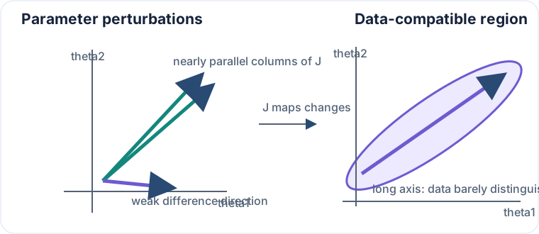
Figure 1:The long axis is not a solver failure. It identifies the combination that the specified measurements leave weakly constrained.
Before solving, identify the map’s units, rank, visible directions, null directions, and the scaling choices that may control its condition number.
Use matrix-vector products where possible, QR for stable least squares, SVD when rank and null directions matter, and covariance-aware weights only when the measurement model warrants them.
Check residuals, reconstruction identities, rank assumptions, singular values, and sensitivity to rescaling. Compare a structured computation with a small explicit dense case.
Continue to What is a derivative?. For Jaxstro’s numerical helpers, see Linear algebra helpers.