An inference begins with a recorded measurement and asks which source states could have produced it through a stated instrument. The answer inherits every assumption in that chain.
The generative chain
A physical model maps parameters and state to ideal observables. A measurement model maps those observables to possible recorded data, including calibration, selection, censoring, and noise. Together they define a likelihood: the probability model for data conditional on parameters and assumptions.
A prior represents information or regularization supplied before the current data. Bayes’ rule combines prior and likelihood into a posterior. A posterior predictive distribution propagates posterior uncertainty into possible observations. A nuisance parameter affects the data model without being the main scientific target; ignoring it does not make its effect disappear.
With parameters , nuisance quantities , and recorded data , Bayes’ rule has the proportional form
The omitted normalizing constant is the evidence for the stated model. A posterior predictive is a distribution for a replicated observation, , after propagating the posterior through the same measurement model. It is not merely the forward model evaluated at one fitted parameter value.
Information has several meanings
Retained scientific detail, stored data volume, Shannon information, and information about parameters are related but not interchangeable. Compression can reduce storage while retaining a model-relative sufficient statistic, or it can destroy the exact structure needed to distinguish models.
Once discarded information is absent from the data product or forward map, no optimizer or sampler can reconstruct it without new assumptions. High Fisher information can imply narrow local uncertainty under a model, while the same analysis remains biased under a misspecified model. A precise posterior is not proof of an adequate model.
Identifiability before computation
Parameters are identifiable only to the extent that distinct values produce distinguishable predicted data under the experiment. Flux and distance, stellar radius and temperature, or calibration and amplitude can create degeneracies. Priors may regularize those directions, but they do not retroactively add information to the likelihood.
Model checking
Posterior predictive checks, residual structure, held-out prediction, and sensitivity to assumptions ask whether model-generated data resemble relevant features of observations. Passing one check supports only the feature and domain tested. Failure can identify useful missing structure rather than merely a bad fit.
Try the running case
For the two-channel measurement, write the path from source parameters to ideal measurements, then to recorded values. Where does a shared calibration offset belong: in the physical model, the measurement model, or the prior? What observation would a posterior predictive replicate?
Worked audit
A shared calibration offset belongs in the measurement model unless a physical argument makes it part of the source. The posterior predictive must replicate recorded measurements, including its calibration and noise assumptions. If it reproduces the fitted mean but misses the correlation between the two calibrated measurements, the likelihood is incomplete for that feature.
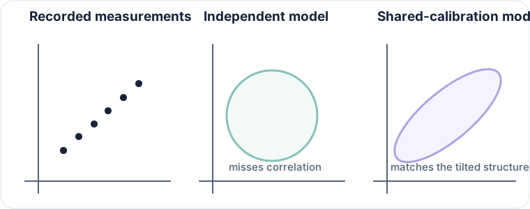
Figure 1:Posterior prediction asks whether replicated recorded data carry the same structure as the observation. Matching a mean while missing the correlation leaves the measurement model incomplete.
Draw the generative chain from parameters and state to observable and recorded data. Mark nuisance quantities, selection effects, assumed independence, and parameter combinations that may be degenerate.
Evaluate the forward and measurement models separately before combining them. Inspect likelihood geometry, parameterization, prior influence, and numerical diagnostics rather than retaining only a posterior summary.
Use simulated recovery, prior predictive checks, posterior predictive checks, held-out observations, residual structure, and alternative parameterizations. Test whether conclusions survive scientifically plausible model changes.
Continue to Sensitivity, conditioning, and identifiability and What is a model?.