The question this method answers
How can a researcher summarize coupled variation, fit a linear model, or solve a dense system without hiding rank and conditioning assumptions? Linear algebra turns vectors of measurements into geometric questions about directions, projections, and sensitivity.
Before computation: what should be true?
State the shapes and units first. For observations and features, a
design matrix has shape and a response has leading shape . A
weighted fit needs finite nonnegative weights of shape . Covariance needs
n_obs - ddof > 0 for unweighted covariance and
sum(weights) - ddof > 0 for weighted covariance. The weighted denominator is
the current frequency-weight-style runtime semantics, not an
effective-sample-size correction. A solve also needs a rank assumption or an
explicit singular-value cutoff.
Define the mathematical objects
A vector is an ordered collection of scalars. Its Euclidean norm is . A matrix is a linear map between vector spaces. Its singular values measure how strongly it stretches different directions; the 2-norm condition number is . Large conditioning means small input changes can produce large solution changes.
Covariance measures joint centered variation. If row is observation and is the sample mean, the unweighted estimator is
The diagonal contains variances. Correlation divides by the two standard deviations, making it dimensionless. A zero variance means that normalization is undefined; Jaxstro returns finite zeros for that row and column rather than inventing a correlation.
Derive the method
The covariance estimator follows directly from centered outer products:
Weighted least squares chooses coefficients to minimize squared residuals :
The implementation does not form the normal equations. It multiplies each row of and by and delegates to JAX least squares, avoiding the extra conditioning penalty of explicitly forming . The normal equation is still a useful audit: should be near zero.
QR factors a tall matrix as with orthonormal columns in , then solves . SVD writes and inverts only singular values above the chosen cutoff.
What the algorithm actually does
covariance_matrix(samples, weights=None, rowvar=False, ddof=1) treats rows as
observations by default. rowvar and ddof are static in its compiled core.
Under the current weighted rule, one observation with weight 2 and ddof=1
passes because its denominator is one and returns a zero covariance matrix. This
illustrates the normalization convention; it is not evidence for two independent
observations.
weighted_lstsq accepts scalar or array-valued responses with the same leading
sample axis. qr_solve requires rows greater than or equal to columns;
svd_solve zeroes inverse singular values at or below rcond * max(s).
positive_definite_jitter scans a fixed geometric sequence of diagonal shifts
and returns (shifted, jitter, success). It returns the first successful tested
shift, not the smallest possible perturbation or a nearest positive-definite
matrix Cheng & Higham (1998).
What JAX differentiates
JAX differentiates the executed dense algebra. Smooth derivatives are useful
while rank, SVD cutoff membership, and the declared zero-weight pattern stay
fixed. A zero weight gives that observation known-zero local sensitivity.
Rank changes, cutoff crossings, zero-norm branches, zero variance, first-success
jitter selection, and coincident singular values are nonsmooth boundaries.
condition_number is a diagnostic, not an inference objective; exact
singularity returns positive infinity.
Table 1:Linear-algebra differentiation contracts
Operation | Supported derivative claim | Boundary |
|---|---|---|
Norm and projection at regular points |
| The active norm or denominator stays nonzero. |
Weighted least squares with fixed full-rank design |
| Rank and the weight pattern stay fixed. |
Zero-weight observation |
| This is declared exclusion, not robust inference. |
QR/SVD solve inside a fixed full-rank/cutoff regime |
| No rank or retained-subspace transition occurs. |
Rank changes, SVD cutoff crossings, and condition numbers |
| Residuals, ranks, and condition diagnostics are audited instead. |
Zero variance and jitter selection |
| Guards and first-success selection are branch boundaries. |
Using it in Jaxstro
from jaxstro.jaxconfig import enable_high_precision

enable_high_precision()

import jax.numpy as jnp

from jaxstro.numerics.linear_algebra import (
    correlation_from_covariance,
    covariance_matrix,
    positive_definite_jitter,
    qr_solve,
    svd_solve,
    weighted_lstsq,
)

x = jnp.array([0.0, 1.0, 2.0, 3.0])
design = jnp.stack([jnp.ones_like(x), x], axis=1)
observations = jnp.array([1.0, 3.0, 5.0, 20.0])
weights = jnp.array([1.0, 1.0, 1.0, 0.0])

unweighted_coeffs = weighted_lstsq(design, observations)
weighted_coeffs = weighted_lstsq(design, observations, weights)
qr_coeffs = qr_solve(design[:3], observations[:3])
svd_coeffs = svd_solve(design[:3], observations[:3])

samples = jnp.array(
    [[1.0, 2.0, 5.0], [2.0, 4.0, 5.0], [3.0, 6.0, 5.0], [4.0, 8.0, 5.0]]
)
covariance = covariance_matrix(samples)
correlation = correlation_from_covariance(covariance)

matrix = jnp.diag(jnp.array([-0.03, 2.0]))
shifted, jitter, success = positive_definite_jitter(
    matrix, initial_jitter=1.0e-3, growth=10.0, max_steps=4
)

assert jnp.allclose(unweighted_coeffs, jnp.array([-1.6, 5.9]))
assert jnp.allclose(weighted_coeffs, jnp.array([1.0, 2.0]))
assert jnp.allclose(qr_coeffs, svd_coeffs)
assert jnp.all(jnp.isfinite(correlation))
assert jnp.allclose(correlation[2], 0.0)
assert success and jnp.isclose(jitter, 0.1)
assert jnp.linalg.eigvalsh(shifted).min() > 0.0
How to audit the result
Check shapes, units, weight domains, and the effective covariance denominator.
Compare with zero and report residuals by observation.
Compare QR and SVD in a well-conditioned full-rank fixture Golub & Van Loan (2013).
Perturb independently and compare central differences with AD while rank is fixed.
Report singular values, the SVD cutoff, selected jitter, and
success.
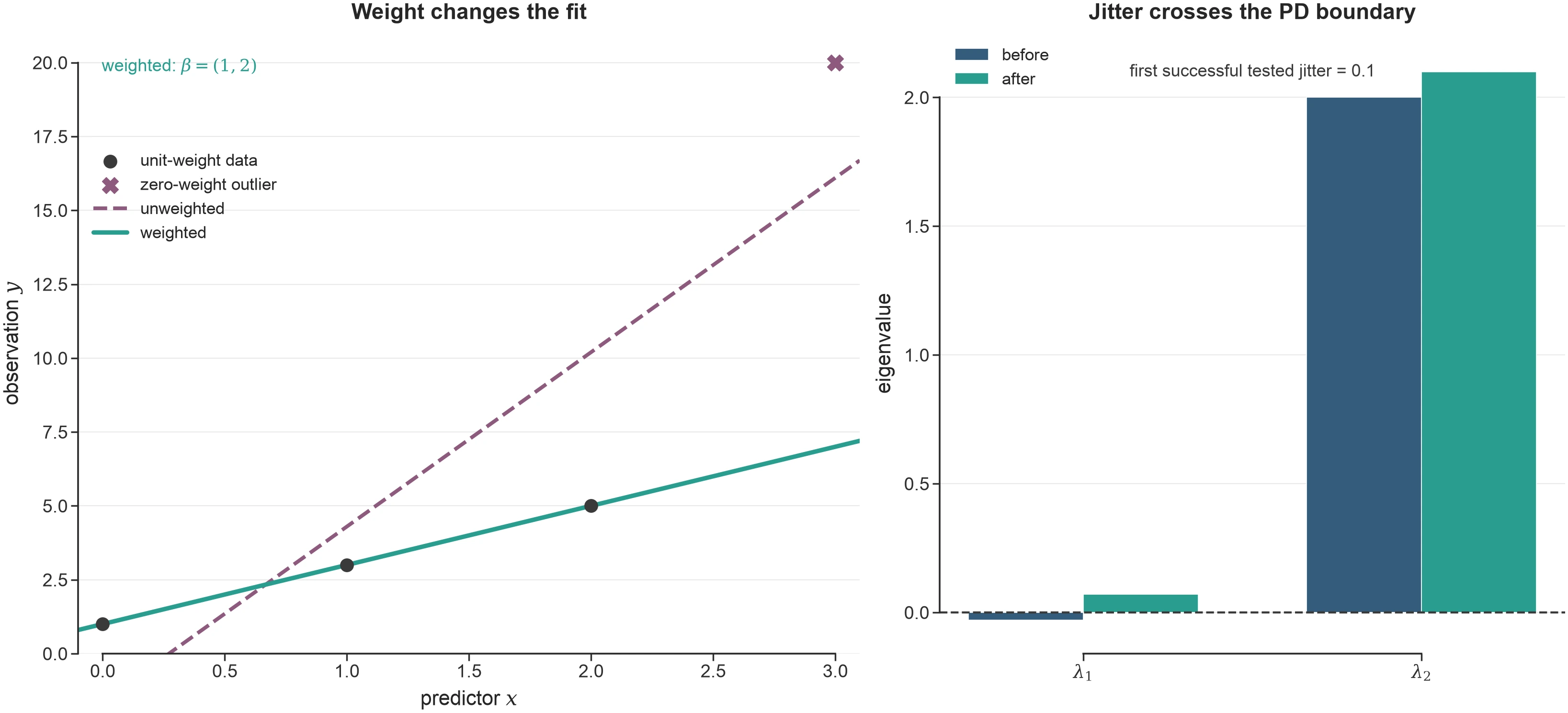
Figure 1:The public APIs produce both panels. This fixed fixture demonstrates declared weighting and jitter policy; it is not a robust-regression benchmark.
Figure 1 ties the reported fit and jitter diagnostics to the concrete fixture used in the audit.
Where the claim stops
These helpers do not establish model adequacy, identifiability, robust outlier policy, or uncertainty calibration. Jaxstro does not own sparse or iterative linear solves here; the delegated Lineax guide remains separate. A finite correlation matrix is not proof that an arbitrary input was symmetric or positive semidefinite.
Connected ideas
- Cheng, S. H., & Higham, N. J. (1998). A Modified Cholesky Algorithm Based on a Symmetric Indefinite Factorization. SIAM Journal on Matrix Analysis and Applications, 19(4), 1097–1110. 10.1137/S0895479896302898
- Golub, G. H., & Van Loan, C. F. (2013). Matrix Computations (4th ed.). Johns Hopkins University Press. 10.56021/9781421407944