Engine B is the density-defined route into
MultiComponentCluster: you prescribe each component’s
density shape (Plummer, EFF, or King density) and its mass-fraction
amplitude, and the engine constructs the one shared self-consistent
potential they jointly generate, recovers each component’s
distribution function by Eddington inversion in that shared
potential, and samples a true joint equilibrium — or refuses, with
the physics named, when the decomposition does not exist as one.
from progenax import MultiComponentCluster, PlummerProfile, EFFProfile

model = MultiComponentCluster.from_density_profiles(
    profiles=[PlummerProfile(r_h=2.0), EFFProfile(a=0.8, gamma=5.0, r_t=9.0)],
    mass_fractions=jnp.array([0.6, 0.4]),   # M_j / M_total, must sum to 1
    m_j=jnp.array([0.5, 1.0]),              # stellar-mass labels (N_frac_j ∝ f_j/m_j)
    r_a_j=None,                              # optional per-component OM radii
)
One quadrature pass, no ODE
The structural contrast with Engine A is this: Engine A’s density is a functional of the potential (the DF defines ), so finding the model requires solving a coupled Poisson ODE. Engine B’s total density is prescribed,
so the shared potential follows from one cumulative-trapezoid pass — no ODE, no iteration:
with the relative potential (so
, increasing inward) and
analytic from the enclosed
mass. The implementation (profiles/density_poisson.py) works in
dimensionless units (, total truncated mass 1) on a fixed
grid — sqrt-stretched toward the core (, audit S2), with non-uniform trapezoid
weights — and stores per-component enclosed-mass CDFs
for the position sampler.
Per-component Eddington inversion in the shared Ψ
Each component’s ergodic DF is the standard Eddington inversion — but performed in the shared relative potential, not the component’s own isolated one:
Two numerical points are load-bearing:
The substitution turns the integrable singularity into a smooth integrand (), which is what makes the quadrature both accurate and gradient-safe.
The truncation boundary term is not optional for truncated models: dropping it corrupts at low binding energies.
The inverter (eddington_invert, in kinematics/eddington.py) was
extracted bit-identically from the validated EFF Eddington table,
so the existing EFF physics suite pins its behavior. Its strongest
truth test bypasses all of progenax’s own potential numerics: fed the
analytic Plummer pair it reproduces the closed-form
law to — with the
untruncated zero point; the truncated case is covered by an exact
closed form including the boundary term, matched to
.
Osipkov–Merritt anisotropy
Per-component radial anisotropy uses the augmented-density device of Merritt (1985): replacing by
in (3) yields with
, i.e. the Osipkov–Merritt anisotropy profile
. Each component carries its own
(inf = isotropic). The sampled anisotropy realizes the
target profile: max
(4 seeds × 20k stars, gate 0.05).
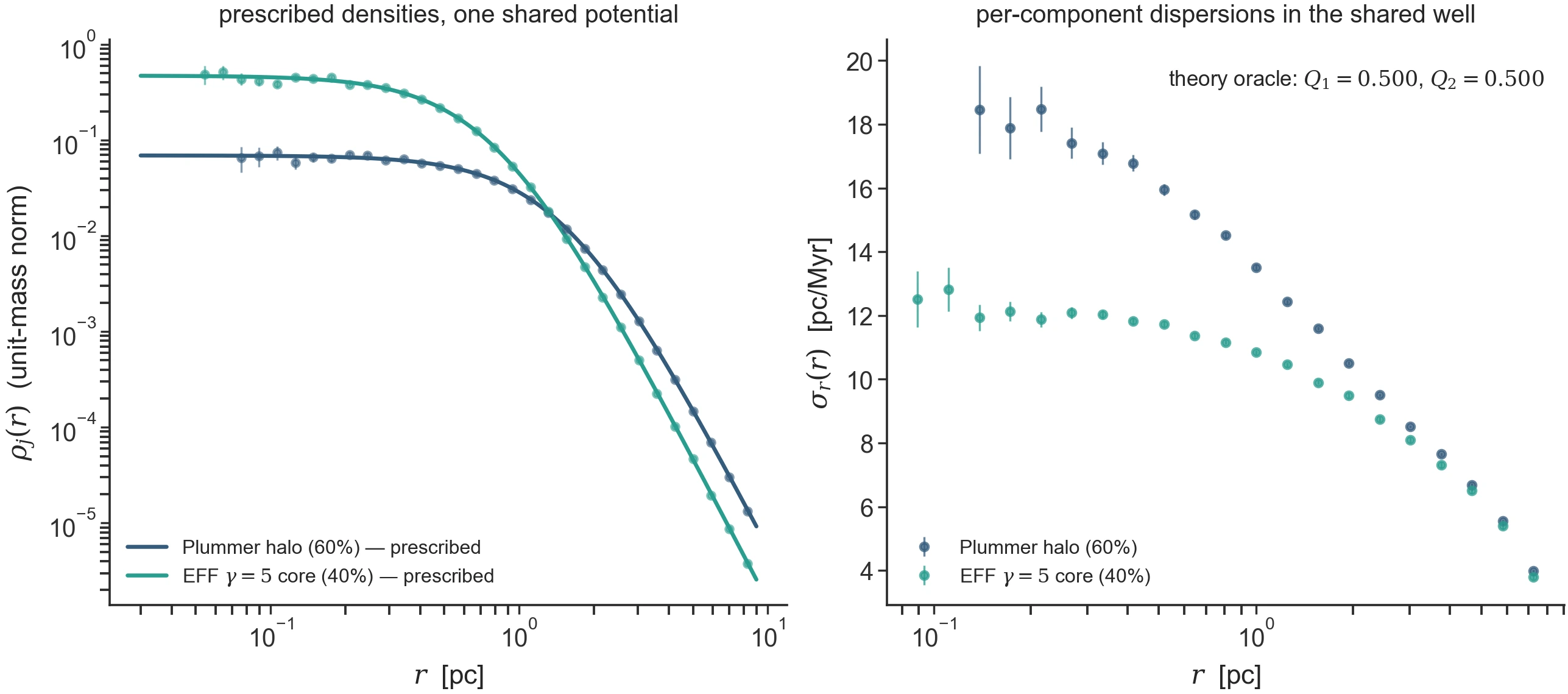
Figure 1:The density-defined route, measured (seed 32, stars): a
Plummer halo (60%) + EFF core (40%) in ONE shared potential.
Left: sampled per-component densities riding the prescribed curves through
the crossover. Right: the same well, two different dispersion profiles —
the halo component is HOTTER at small (its wide-orbit stars pass through
the core), a pure shared- Eddington effect; the theory oracle reads
. Regenerate: python -m laboratory.icviz --only engine-b-mix.
Derived domains (the model decides, never the code)
A component’s radial extent is part of the prescribed model, so the cluster truncation radius is derived, with the rule that set it stored as provenance:
Component extents: Plummer is infinite; EFF and King end at their own .
Cluster edge = max finite extent. If any component is finite, is the largest finite extent (provenance names the winning profile and component index).
All-infinite mixes (e.g. pure Plummer): is the radius enclosing (configurable) of the summed analytic mass, found by a fixed 80-step bisection.
Explicit
r_t=override wins — except that an override which would re-truncate a King component below its natural edge raises aValueError: a King model’s lowered-Maxwellian edge is prescribed physics, never silently cut.
Per-component truncated-mass fractions are stored as diagnostics, so a “too small ” cannot hide.
The realizability gate: or refuse
Eddington inversion is the unique candidate ergodic (or OM) DF for a density in a potential. If that candidate is negative anywhere, the prescribed component does not exist as an equilibrium in this shared potential — typically a too-shallow component in a concentrated companion’s potential. Engine B treats this as physics:
Every build computes and stores the margin per component.
Genuine negativity (, separating physics from grid-level quadrature ringing) on a concrete build raises a
ValueErrornaming the component and the remedy (“density too shallow to be supported in this shared potential — steepen it, raise its mass fraction, or raiser_a_j”).Traced builds (under
jax.jit/jax.grad) cannot raise, so they always store thef_min_jdiagnostic instead — the same two-tier patternEFFVelocityDFuses.The DF is never clamped silently: a clamped DF integrates back to a different density than the one prescribed.
This is not a corner case. The originally drafted halo+core example ( inside a Plummer halo) is genuinely unrealizable (, resolution-independent), with the gate flip measured between and 0.68 — see the worked example for the full story.
What the DF can and cannot represent
The Eddington pair represents : any constant edge offset is invisible to an ergodic DF. A hard-truncated prescribed density has , and no can carry that offset; with OM anisotropy the unrepresentable offset is amplified by the augmentation factor . The consequence is a small, predictable deficit between the DF-reconstructed density and the prescribed near the edge. Interior fidelity is gated: (OM build) and (isotropic) inside the component half-mass radius, against a gate.
Hybrid sampling and the predict-the-offset 
sample_cluster for an Engine B model is a hybrid: positions come
from the prescribed (per-component inverse-CDF on
), speeds from the component’s table at the star’s
, directions from the OM stretched split at the star’s
component , and the velocity scale from the actual sampled
mass (never an independent input total — energies must
use the realized cluster mass). There is no external virial
rescale.
Because of the edge-offset physics above, a hard-truncated component’s
sampled plateaus slightly below 0.5 — and Engine B predicts
the plateau with an exact-quadrature hybrid expectation (prescribed-ρ
weights × DF speed moments × prescribed-total Clausius field):
predicted , sampled over 18
seeds — verified truncation-edge physics, gated against the
prediction. The pure-DF theory oracle (component_virial_ratios,
which weights by — the density the DF actually
represents) reads to a few , as the
steady-state identity demands. Do not rescale Engine B output to
“fix” the plateau.
A numerics lesson: never differentiate interpolated data
The King-density branch initially computed
by jnp.gradient of the interpolated King grid. Piecewise
linear interpolation makes that derivative a staircase, and the
Eddington kernel plus the Abel
weight focus the staircase ringing exactly into
— a single King component (whose true ergodic DF
is strictly positive) read , squarely inside the
realizability gate’s field of view. The fix integrates King’s own
Poisson identity,
by cumulative trapezoid of the closed-form density — after which . The general rule is worth the emphasis: in any Abel-type inversion, differentiate closed forms or exact identities, never interpolated data.
Check yourself
1. Why is the halo hotter in the core?
In Figure 1 both components share one , yet . Explain via the Eddington construction: a shallower requires a hotter to be self-consistent in the same well — the halo’s stars seen at small are passing through on wide, energetic orbits.
2. Make the gate refuse
Rebuild the mix with the EFF core shrunk to . The Eddington candidate DF for the halo goes genuinely negative (, resolution-independent) and construction raises with the physics named — see Two-component populations — worked examples for why, and where the realizable boundary sits (–0.68).
Validation summary
All anchors from scripts/validate_multicomponent_eddington.py
(11/11 PASS); the full evidence page is at
Multi-component Eddington equilibria (Engine B).
Engine B measured anchors (2026-06-10 close-out).
Check | Measured | Gate |
|---|---|---|
King A-vs-B radial KS distance (two independent engines, ) | ||
King A-vs-B max (interior bins) | ||
Plummer (untruncated zero point) | ||
Plummer vs exact truncated closed form | ||
Halo+core theory (DF-weighted oracle) | ||
Halo+core sampled global (, unscaled) | 0.4976 | |
Hard-truncated halo vs hybrid prediction | sampled vs predicted 0.4953 | |
OM realization (max deviation) | 0.028 | |
DF-density fidelity, interior (OM / isotropic) | / | |
AD-vs-FD gradients (, mass-fraction , ) | / / |
The King anchor deserves emphasis: a single King component is the only
configuration both engines describe identically (Engine A at ;
Engine B from the King density), through entirely disjoint numerics
(coupled ODE + lowered-DF sampling vs. quadrature potential +
Eddington inversion). Their agreement at the 10-4 level is the
cross-engine trust statement for the whole
MultiComponentCluster design.
Differentiability
The build is differentiable in the profile parameters (e.g. halo
), the mass fractions (via a reparametrized scalar), and the
— AD matches finite differences to
(table above). Two deliberate exceptions: the domain choice
(derive_r_t) concretizes — picking which component’s extent wins is
a construction-time decision, not differentiated through — and the
King component’s internal subgraph (its own ODE solution) is
constant with respect to the differentiated parameters.
Implementation, validation & references
In code: the shared-potential quadrature is
src/progenax/profiles/density_poisson.py, the ergodic/OM inverter iseddington_invertinsrc/progenax/kinematics/eddington.py, and the Engine-B constructor isMultiComponentCluster.from_density_profilesinsrc/progenax/cluster/multicomponent.py. See the cluster API.Validated in: Engine B (Eddington) — the 11-anchor close-out (A-vs-B trust anchor, , realizability, OM , AD-vs-FD gradients) summarised above.
Primary sources: Eddington inversion is standard ergodic-DF machinery; the augmented-density Osipkov–Merritt construction is Merritt (1985). The density components are Plummer Plummer, 1911, EFF Elson et al., 1987, and King King, 1966; the DF-defined counterpart is the Gieles & Zocchi (2015) family (Engine A). Full notes in the bibliography.
- Merritt, D. (1985). Spherical stellar systems with spheroidal velocity distributions. The Astronomical Journal, 90, 1027–1037. 10.1086/113810
- Plummer, H. C. (1911). On the problem of distribution in globular star clusters. Monthly Notices of the Royal Astronomical Society, 71, 460–470. 10.1093/mnras/71.5.460
- Elson, R. A. W., Fall, S. M., & Freeman, K. C. (1987). The structure of young star clusters in the Large Magellanic Cloud. The Astrophysical Journal, 323, 54–78. 10.1086/165807
- King, I. R. (1966). The structure of star clusters. III. Some simple dynamical models. The Astronomical Journal, 71, 64–75. 10.1086/109857
- Gieles, M., & Zocchi, A. (2015). A family of lowered isothermal models. Monthly Notices of the Royal Astronomical Society, 454, 576–592. 10.1093/mnras/stv1848