The question this method answers
Given values known only at ordered coordinates, what value should represent the table between samples? Interpolation fills finite gaps under an explicit shape assumption. It does not discover unresolved physics or justify extrapolation.
Before computation: what should be true?
The coordinate array must be one-dimensional, contain at least two points, and be strictly increasing. The selected value axis must have the same length. State whether the data justify linearity, smooth curvature, known node derivatives, or monotone shape. Choose clamping or extrapolation before computing.
The meaning of coordinate units and scales is developed in Functions, units, and scales; table payloads connect to Scientific representations.
Define the mathematical objects
Let be knots and let be scalar samples. The linear, Hermite, and PCHIP implementations also allow array-valued payloads along a selected axis; the natural-cubic implementation does not. For a query , define the interval width and local coordinate . Node derivatives are denoted and secant slopes are .
A boundary policy specifies the value outside $[x_0,x_{n-1}]`: clamp to endpoint values or numerically continue the endpoint segment. A limiter branch is the piecewise rule that chooses monotone cubic slopes from neighboring secants.
Derive the method
The unique straight line through two adjacent samples is
To match both endpoint values and endpoint derivatives, use the cubic Hermite basis:
where
For monotone PCHIP slopes, adjacent secants with different signs imply a zero node derivative. Otherwise Fritsch & Butland (1984) gives the weighted harmonic mean
Endpoint slopes receive additional sign and three-times-secant limiters. These branches prevent a monotone table from gaining a new interior extremum.
The natural cubic instead solves for knot second derivatives with and
This creates a globally interpolant, but it need not preserve monotonicity or remain inside the sample range Boor (2001).
What the algorithm actually does
interp1d locates intervals with searchsorted, computes (1),
and defaults to endpoint clamping. cubic_hermite_interp evaluates supplied
derivatives. pchip_slopes constructs limited slopes, and
monotone_cubic_interp passes them to the Hermite evaluator. Natural-cubic
coefficient construction uses jnp.linalg.solve; eval_cubic_spline evaluates
the selected interval in nested polynomial form and clamps its query first.
Array-valued payloads are supported by the linear, Hermite, and PCHIP paths.
By contrast, natural_cubic_spline_coeffs, eval_cubic_spline, and
NaturalCubicSpline1D support scalar one-dimensional y only. The current
natural-cubic coefficient routine does not cleanly reject an array-valued y;
it reaches incompatible core array assembly and raises TypeError. Treat that
failure as a limitation, not as array-payload support.
Concrete wrappers check the shapes they explicitly support and strictly
increasing grids. Value-dependent exceptions cannot fire on
tracers: eager validation is skipped while the grid is traced; the caller must supply a strictly increasing grid under jax.jit.
With extrapolate=True, the endpoint linear or Hermite segment is numerical continuation, not a physical guarantee.
What JAX differentiates
Table 1:Interpolation gradient contracts
Operation | Contract | Supported claim | Boundary |
|---|---|---|---|
Hermite values and supplied derivatives |
| AD agrees with finite differences in a fixed segment. | The query remains away from knots and clamping. |
Natural-spline values and interior query |
| For scalar one-dimensional | The selected interval remains fixed. |
PCHIP inside a fixed limiter branch |
| AD applies while secant signs and limiter decisions do not change. | A limiter transition changes the executed derivative rule. |
Clamped exterior query |
| Endpoint output is locally constant in the exterior query. | Saturation is not an inference direction. |
Knots and limiter transitions |
| Values, bounds, and one-sided behavior can be checked. | No universal smooth derivative is claimed. |
Using it in Jaxstro
from jaxstro.jaxconfig import enable_high_precision

enable_high_precision()  # before creating JAX arrays

import jax.numpy as jnp

from jaxstro.numerics.interpolation import (
    MonotoneTabulatedFunction1D,
    cubic_hermite_interp,
    eval_cubic_spline,
    monotone_cubic_interp,
    natural_cubic_spline_coeffs,
    pchip_slopes,
)

x_grid = jnp.arange(5.0)
values = jnp.array([0.0, 0.01, 0.9, 0.91, 1.0])
x_new = jnp.linspace(0.0, 4.0, 801)
dydx = pchip_slopes(x_grid, values)

hermite = cubic_hermite_interp(x_grid, values, dydx, x_new)
natural = eval_cubic_spline(
    x_grid,
    natural_cubic_spline_coeffs(x_grid, values),
    x_new,
)
monotone = monotone_cubic_interp(x_grid, values, x_new)
table = MonotoneTabulatedFunction1D(x_grid, values)
wrapped_monotone = table(x_new)

assert natural.min() < -0.1
assert monotone.min() >= -1e-12
assert monotone.max() <= 1.0 + 1e-12
assert jnp.all(jnp.diff(monotone) >= -1e-12)
assert jnp.allclose(hermite, monotone)
assert jnp.allclose(wrapped_monotone, monotone)
Prepared TabulatedFunction1D, MonotoneTabulatedFunction1D, and
NaturalCubicSpline1D objects are registered PyTrees. Their table arrays are
dynamic leaves; interpolation axes stored by the monotone wrapper are static
auxiliary data. This PyTree behavior does not widen NaturalCubicSpline1D
beyond its scalar one-dimensional value contract.
How to audit the result
Check exact reproduction at every knot, then probe midpoints. For monotone data, audit output range and successive increments. For a smooth analytic function, refine the grid and compare errors. Compare AD with central finite differences only at interior queries whose interval and limiter branch remain fixed.
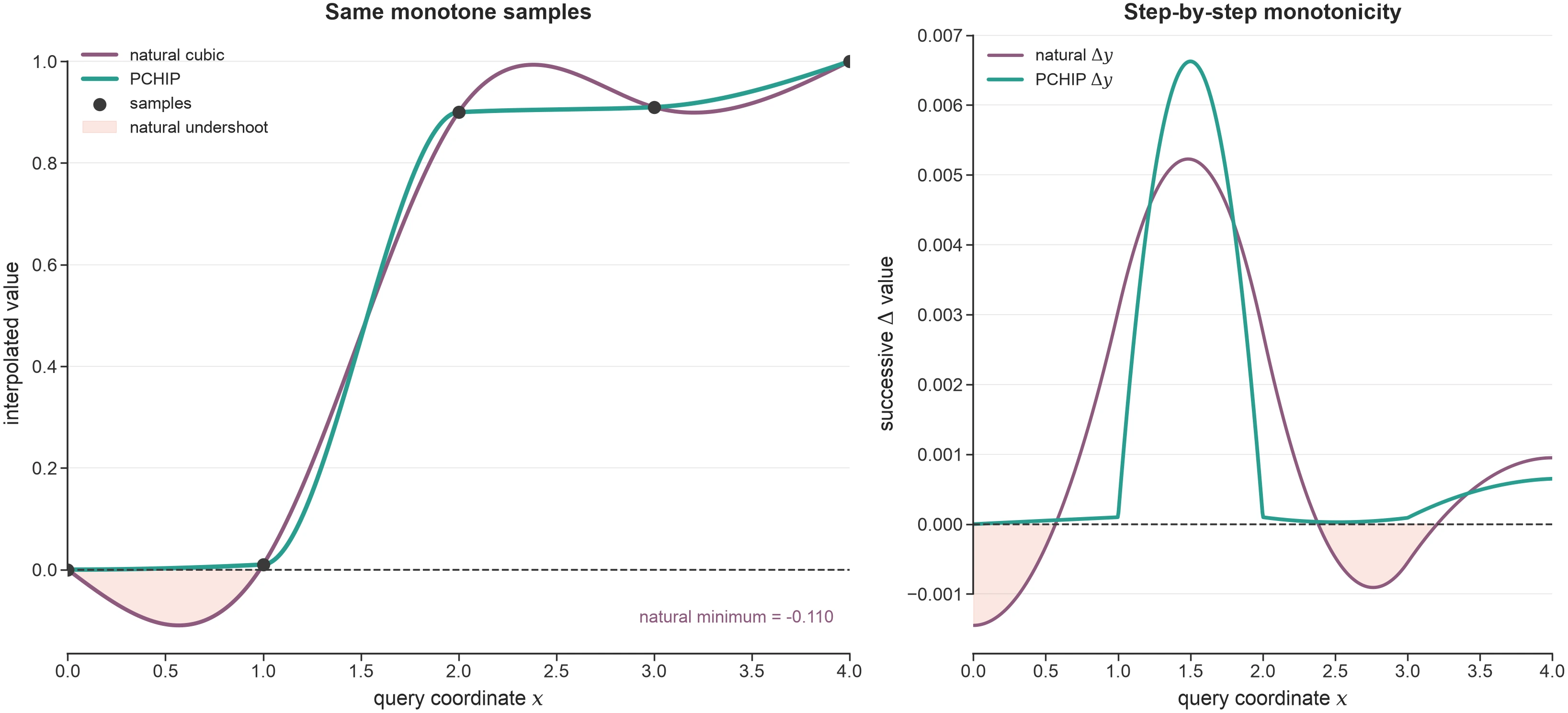
Figure 1:The same monotone samples demonstrate that natural-cubic smoothness and PCHIP shape preservation are different contracts, not a universal ranking.
Executable anchors are indexed in Validation. Figure 1 makes the distinction between the two interpolant contracts visible on the same samples.
Where the claim stops
These are one-dimensional table primitives. They do not estimate interpolation error, infer missing structure, validate a table’s physical meaning, or handle scattered data and multidimensional monotonicity. PCHIP preserves monotone shape for monotone samples; it does not make noisy or biased data correct.
Connected ideas
- Fritsch, F. N., & Butland, J. (1984). A Method for Constructing Local Monotone Piecewise Cubic Interpolants. SIAM Journal on Scientific and Statistical Computing, 5(2), 300–304. 10.1137/0905021
- de Boor, C. (2001). A Practical Guide to Splines (Vol. 27). Springer New York. 10.1007/978-1-4612-6333-3