The question this method answers
How can a smooth function be represented by local basis functions so that one coefficient changes only a limited region? A degree- B-spline writes using knots, local basis functions, and coefficients.
Before computation: what should be true?
The knot vector must be one-dimensional, nondecreasing, long enough for the nonnegative integer degree, and define a positive-width active domain. The coefficient axis must have length . Decide whether knots are fixed representation choices or data-dependent preprocessing.
Basis vectors are a linear representation; see Linear algebra as the language of change and Scientific representations.
Define the mathematical objects
Let be knots, the polynomial degree, and the th normalized basis function. Its support is contained in . Inside the active domain, bases are nonnegative and form a partition of unity. A clamped open knot vector repeats each endpoint times.
The coefficient vector defines . A design matrix has entries . A derivative-order- roughness functional measures the integrated square of .
Derive the method
The degree-zero basis selects one half-open knot interval:
The Cox-de Boor recurrence builds higher degree from adjacent lower-degree bases Boor (1972):
A zero denominator contributes zero, which is the standard repeated-knot convention. Differentiating the spline gives a degree- spline with
The coefficient sensitivity is especially simple: . For smoothing, Jaxstro approximates
on a fixed sample grid. A caller may form an objective such as , but remains caller-owned.
Antiderivative increments obey
enabling definite integrals by endpoint subtraction.
What the algorithm actually does
bspline_basis evaluates (2) for every basis and clamps queries
to the active domain. bspline_eval contracts coefficients with that basis;
bspline_eval_deboor provides the equivalent local de Boor evaluator.
bspline_derivative, bspline_antiderivative, and bspline_integral transform
coefficients and knot vectors as above.
open_uniform_knots creates clamped equally spaced interior knots.
adaptive_open_uniform_knots places interior knots at sample quantiles; this is
deterministic preprocessing, not knot optimization. fit_bspline_lstsq solves
ordinary fixed-knot least squares. tensor_product_design_matrix computes a
row-wise Kronecker product. Degree and relevant axes are static under JIT.
Invalid concrete degree, knot order, coefficient shape, sample shape, or active
domain raises ValueError. Value-dependent knot checks cannot raise while the
knots are traced.
What JAX differentiates
Table 1:B-spline gradient contracts
Operation | Contract | Supported claim | Boundary |
|---|---|---|---|
Coefficients at fixed knots |
| AD returns the active basis vector. | Knots and degree remain fixed. |
Interior query coordinate |
| AD agrees with finite differences in a smooth knot span. | Query stays away from repeated knots and boundaries. |
Clamped exterior coordinate |
| Evaluator and analytic derivative are constant outside. | Saturation is not an inference direction. |
Knot boundaries |
| Multiplicity-specific continuity can be checked. | No universal knot gradient is claimed. |
Quantile knot construction |
| Deterministic placement can be reproduced. | Sorting and quantiles are preprocessing boundaries. |
Using it in Jaxstro
from jaxstro.jaxconfig import enable_high_precision

enable_high_precision()  # before creating JAX arrays

import jax.numpy as jnp

from jaxstro.numerics.splines import (
    BSpline1D,
    bspline_basis,
    bspline_derivative,
    bspline_eval,
    open_uniform_knots,
)

knots = open_uniform_knots(0.0, 1.0, n_basis=6, degree=3)
coeffs = jnp.array([0.0, 0.25, 0.9, 0.7, 0.2, 0.1])
x = jnp.linspace(0.0, 1.0, 9)

basis = bspline_basis(knots, x, degree=3)
values = bspline_eval(knots, coeffs, x, degree=3)
derivative = bspline_derivative(knots, coeffs, x, degree=3)

spline = BSpline1D(knots, coeffs, degree=3)
wrapped_values = spline(x)

assert basis.shape == (9, 6)
assert jnp.allclose(basis.sum(axis=-1), 1.0)
assert jnp.allclose(values, wrapped_values)
assert jnp.all(jnp.isfinite(derivative))
How to audit the result
Check basis nonnegativity, local support, and partition of unity. Compare basis contraction against de Boor evaluation. Verify AD with respect to coefficients against the basis vector and AD with respect to an interior query against both the analytic derivative and central finite differences. For a fit, inspect design rank, condition, residuals, and sensitivity to knots and regularization.
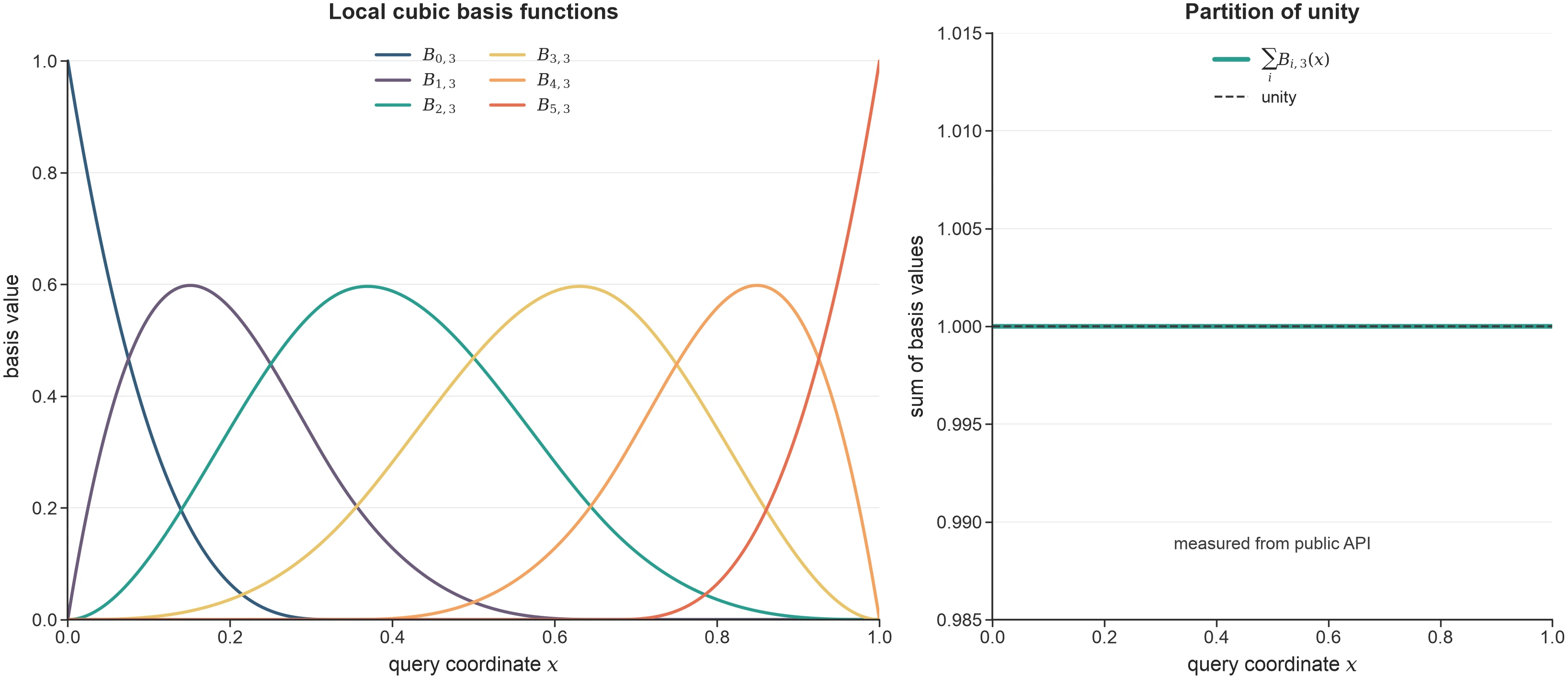
Figure 1:The public basis values show local support and partition of unity for one open-uniform cubic configuration. They do not validate knot or smoothing-model selection.
Measured anchors are indexed in Validation. Figure 1 is the visual check for the local-support and partition-of-unity behavior described above.
Where the claim stops
Jaxstro does not own smoothing-spline model selection, adaptive-knot optimization, extrapolation, sparse tensor-product storage, uncertainty calibration, or a domain-specific regularization policy. Deterministic quantile knots are not an optimized adaptive spline.
Connected ideas
- de Boor, C. (1972). On calculating with B-splines. Journal of Approximation Theory, 6(1), 50–62. 10.1016/0021-9045(72)90080-9