OED for robustness — when binaries lie to your mass estimate (Stage 4)
The first OED demo whose headline is a BIAS, not a recovery — a binary-blind survey design over-weighs a cluster by 184% with 41× false confidence, and a binary-aware design removes it
The three OED demos before this one each end with the optimiser rediscovering a piece of physics: anisotropy wants the outskirts, concentration wants the core, dynamical mass wants an interior depth. Each is a clean result — and each is one a referee could wave away as “Fisher-OED recovers the obvious.” This page is different. Its headline is not a recovery; it is a bias. We hand a careful, binary-blind observer the optimal survey design for weighing a cluster, let the real cluster harbour the binaries that every real cluster has, and watch the analysis over-estimate the mass by 184% while reporting a 4.5% error bar — a measurement that is confidently, expensively wrong. Then we show the design that protects against it.
Reading paths
Already comfortable with Fisher OED? Skip to the physical question for the binary-systematic science, or jump straight to the headline figure and Quantitative results.
Want the machinery first? Read the OED formalism page, then come back here.
Why does this demo exist at all? It converts OED from “recovers the obvious” into a referee-resistant bias result — see why this arc exists.
Why this arc exists: a bias a referee cannot dismiss
The sibling OED demos are strong engineering — one differentiable Fisher backbone, re-pointed at three science targets — but each headline is either already-known physics or contingent on an arbitrary RV/PM error split that flips with the budget. None is a result a referee couldn’t read as “of course the optimiser put the proper motions where the signal is.”
This demo monetises a capability nobody else has wired to OED: progenax carries a
faithful, differentiable Moe & Di Stefano (2017) binary-population engine, so we can ask the
question that actually bites in real cluster mass measurements — what does an unmodelled
population systematic do to an “optimal” design, and what design defends against it? The
answer is a parameter bias larger than its own forecast uncertainty, which is the one
kind of result a Fisher-OED demo cannot be accused of staging. It is the canonical binary
systematic of dwarf-galaxy and young-cluster dynamics, turned into a design problem.
The physical question: why binaries masquerade as mass
You weigh a star cluster with the virial theorem: a hotter cluster — larger line-of-sight velocity dispersion — is a heavier one, . That logic has a silent assumption: that every velocity you measure is a single star orbiting the cluster. It is not. A large fraction of massive stars live in binaries, and in a single-epoch radial-velocity survey you cannot resolve the binary — you measure the star’s orbital velocity around its companion folded into its cluster velocity. Those orbital motions are fast (tens of km/s for short-period massive binaries), so they inflate the measured dispersion above the true cluster value.
The inflation is not noise — noise averages out. It is a systematic offset in the second moment. If the cluster’s true dispersion is and a fraction of the stars carry a binary velocity drawn from a population with variance , the observed dispersion-squared is
a flat pedestal added on top of the real cluster heat at every radius. Feed to a virial analysis that does not know about the pedestal, and the analysis reads the extra dispersion as extra mass. For our young-massive-cluster fiducial the pedestal is km/s sitting under a central cluster dispersion of only 9.0 km/s — and the cluster term falls to 0.4 km/s in the outskirts, while the pedestal does not budge. That is the whole story: in the cold outskirts the binary pedestal dominates the signal.
The intuition the optimiser is about to fall for — and then defeat
Hold one fact in mind: the cluster mass scales the dispersion amplitude and shows up at every radius; the binary fraction adds a flat offset. The only thing that tells them apart is radial leverage — the cluster dispersion has a shape that falls from core to edge, while the binary pedestal is flat. A design that ignores binaries chases the loudest signal into the cold outskirts and parks its budget exactly where the pedestal is largest relative to the cluster — and so confuses pedestal for mass most badly. A design that models binaries instead spends its stars on the core↔outskirts contrast that breaks the degeneracy. Same instrument, same budget, opposite outcome.
Inputs and assumptions
The design optimises a fixed budget of radial-velocity measurements allocated across log-spaced projected-radius bins — RV only, single-epoch. The science target is the dynamical mass ; the EFF shape parameters are photometrically pinned nuisances, and the anisotropy radius and binary fraction are kinematic nuisances the radial allocation must disentangle. Everything is computed pre-data — the cross-model Monte Carlo afterwards is a calibration gate, not part of the design loop.
Model inputs
Input | Meaning and role | Status (fiducial) |
|---|---|---|
Total dynamical mass — the science target; scales the cluster dispersion amplitude. c-optimality minimises its marginal variance. | target (; index 0 of , no prior) | |
Osipkov–Merritt anisotropy radius — a kinematic nuisance with a weak (50% fractional) prior; the RV-only degeneracy is regularised by it. | nuisance ( pc; index 1; ) | |
EFF outer slope — the concentration shape knob. Photometrically pinned (measured from the surface-brightness profile). | nuisance (; index 2; tight 10% prior) | |
EFF scale radius — parameterised directly (EFF is natively with no closed-form inversion; see the modelling choice). Photometrically pinned. | nuisance ( pc; index 3; tight 10% prior) | |
Binary fraction — the misspecification axis. In the binary-aware model it is a free nuisance with a weak (50%) prior, recovered from radial leverage; in the binary-blind model it is silently fixed at 0. | truth 0.5 (index 4; weak prior or absent) | |
Variance of the single-epoch binary velocity blend — a build-once population scalar from the Moe & Di Stefano –– engine over a Maschberger massive-primary IMF with ZAMS flux weights. | fixed ( (km/s) km/s) | |
density model | EFF (Elson–Fall–Freeman), projected under Osipkov–Merritt. Analytic density no ODE / no OOM (see the modelling choice). | held fixed (the misspecification CONTROL) |
kinematic channel | RV only () — no proper motions, no channel split (the binary systematic lives in the RV second moment; the dwarf/cluster regime). | fixed (the design allocates stars among radii) |
Per-star RV error, entering the per-datum variance . | fixed ( km/s) | |
bins, budget, optimiser | log-spaced bin centres pc; pc; multi-start Adam over the softmax simplex. | numerical choices |
units, |
| known / fixed |
The Fisher is built in the dimensionless metric Important, so is a fractional precision. The pinned scales are the load-bearing ones: km/s and km/s, a contamination ratio at the centre — rising to in the outskirts, because the cluster term collapses while the pedestal stays flat. That the binaries rival the cluster heat at this operating point is pinned before any inference, exactly so that H1 below has a chance to bite.
The modelling choice: EFF-OM, RV-only, and a held-fixed cluster
Two facts about the forward model set up the whole demo, and stating them plainly is the honest way to read the result.
EFF density is analytic — no ODE, no OOM. The Elson–Fall–Freeman profile has a closed-form density , so
project_dispersiondoes a plain quadrature with no differential-equation solver in the tape. This is what makes the cross-model Monte Carlo runnable — the King/Michie ODE solvers in the concentration demo forced its Michie calibration to OOM at 28 GB. The EFF slope doubles as a concentration knob, so the bias vector spans with no ODE anywhere. We parameterise by the EFF scale radius directly rather than a derived half-mass radius, because EFF has no closed-form and inventing one would inject a spurious unpinned inversion.The cluster forward model is the held-fixed CONTROL. This is a misspecification study, and a misspecification study is only clean if it changes one thing. So the EFF-OM cluster model — density shape, OM anisotropy law, RV projection — is identical between the design, the truth, and both fits. The only difference between the “disaster” and the “fix” is whether the analysis models the binaries. Every number on this page is the cost of that one omission, with the cluster physics deliberately frozen so it cannot be blamed.
The method, specialised: c-optimality with a misspecified vs marginalized Fisher
This demo pours the additive backbone
Equation into a c-optimal-for- radial allocation, exactly as the
sibling designs do. One jacrev of the cluster term at the truth gives the per-bin Jacobian
(reverse-mode by policy); the design
enters only through the per-bin counts. The criterion minimises the variance with the
nuisances profiled out:
The whole demo is the contrast between two Fishers built on this one equation:
Binary-blind (, no ): the observer who does not know binaries exist. Its Fisher omits the column entirely.
Binary-aware / marginalized (): adds the column (the pluggable Fisher block) and profiles out as a free nuisance.
Because the Fisher is additive and design-linear, the expensive projection is differentiated
once; the grid for the maximin criterion below only updates the
denominator — no re-jacrev.
The headline (H1): a confident, expensive, wrong mass
The pre-registered hypothesis (H1, locked before the Monte Carlo ran) was: fitting the binary-blind model to binary-contaminated RV data biases high, by more than the design’s own forecast — false confidence. The rival H0 was that the binary-blind fit would absorb the flat pedestal into its nuisances and stay unbiased. H1 is confirmed, decisively.
The binary-blind c-optimal-for- design, fit with the binary-blind model on mock catalogues that do contain Moe binaries, recovers
The estimate is nearly triple the truth, and the design’s own error bar — the precision it promised — is 41 times smaller than the error it actually made. This is the worst failure mode in inference: not a wide error bar (which warns you), but a tight one around the wrong answer.
The control is what makes it airtight. Run the same design and fit on mocks with — where the fit model exactly matches the generative model — and the bias is , well inside the forecast. The entire is the binaries; nothing else moved.
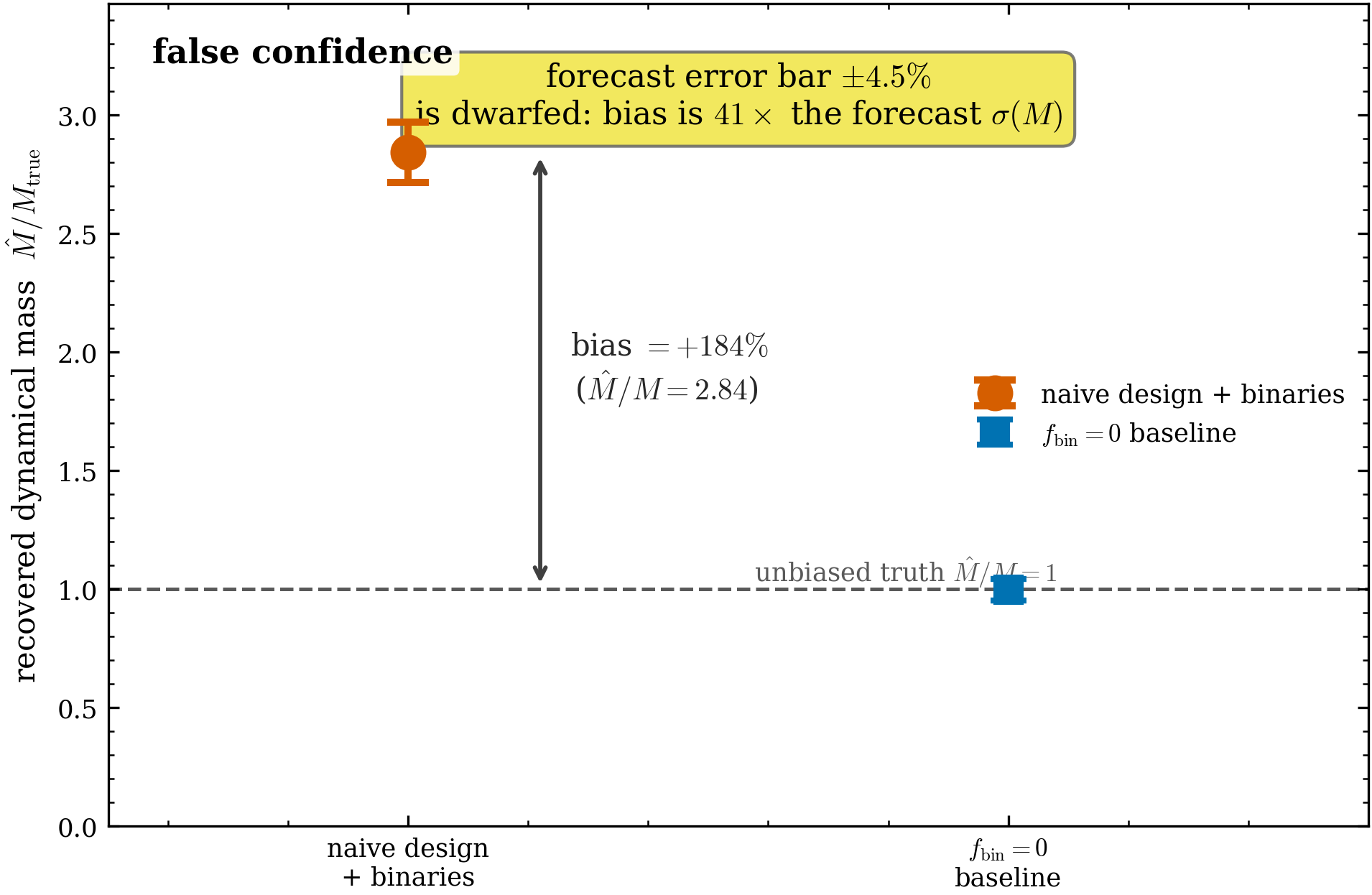
False confidence: a binary-blind design weighs the cluster at its true mass with a error bar. The recovered for the binary-blind c-optimal-for- design fit on binary-contaminated mocks (vermilion, ), drawn with its own ±forecast- error bar — visually a speck. The unbiased truth is the dashed line at 1; the baseline (blue square, mock fit model) recovers . The bias () is annotated against the truth; the callout states the headline — the claimed error bar is smaller than the bias. From the env-gated cross-model Monte Carlo (48 draws).
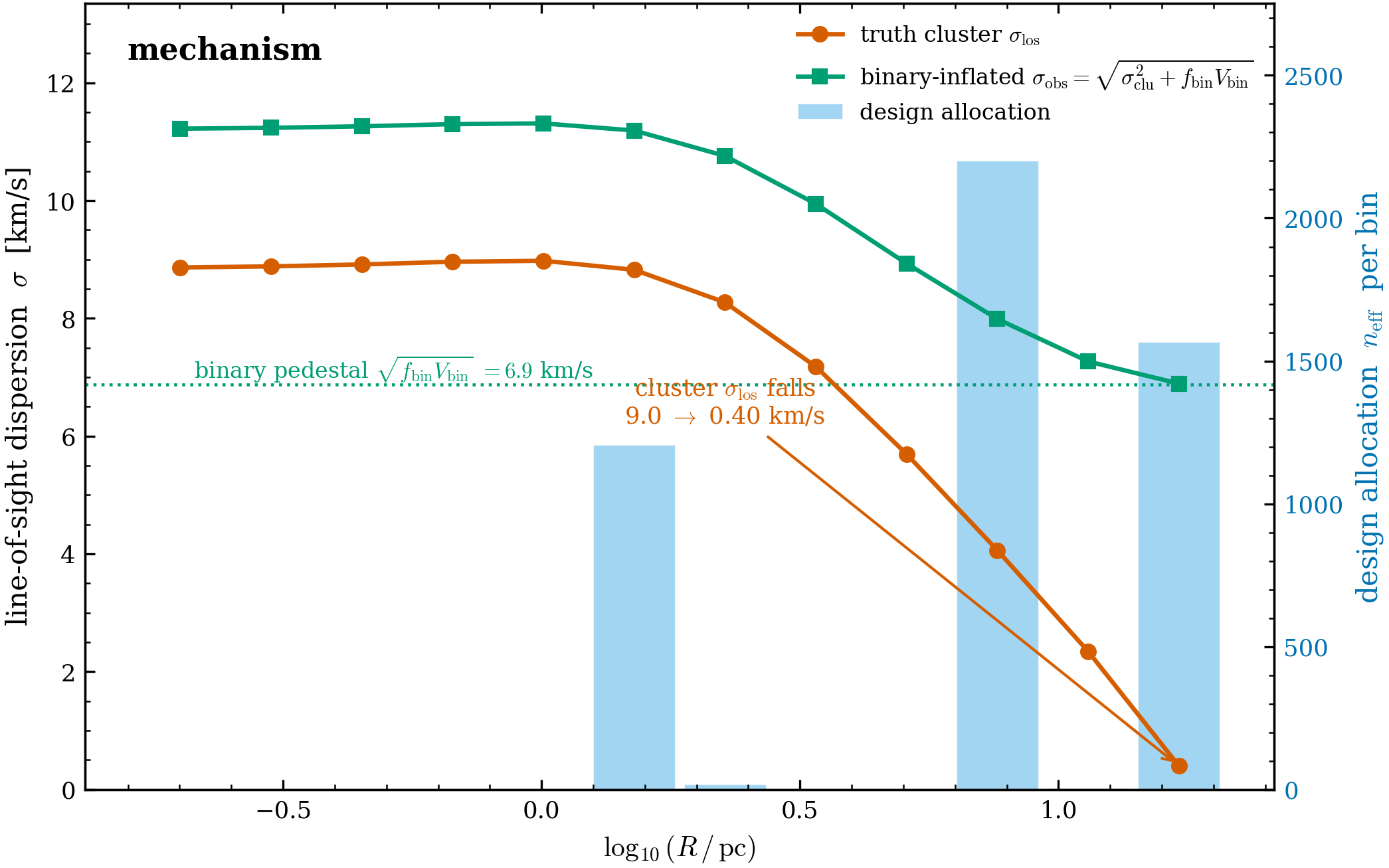
Why it happens: the design parks its budget in the contaminated outskirts. The truth cluster (vermilion) falls steeply from 9.0 km/s in the core to 0.40 km/s at the edge — that fall is the mass signal. The binary-inflated observable (green) sits on a near-flat pedestal at the km/s floor (dotted). The binary-blind design’s per-bin allocation (blue bars, right axis) piles into the outer bins — exactly where the pedestal dominates the signal — so the binary-blind fit reads the pedestal as extra mass. The design optimised for under the wrong model finds the worst possible place to spend its stars.
The fix (measure-and-marginalize): model the binaries, recover them, lose the bias
The remedy is not to throw away the outskirts; it is to model the pedestal. Add the parameter to the fit (and to the design Fisher), let the data determine it, and the bias collapses:
Bias: . The binary-aware fit on the same contaminated mocks recovers within its honest forecast — the cross-model residual bias is consistent with zero (, inside of the marginalized forecast).
It recovers the binary fraction: . Not from a prior — from radial leverage alone. The flat pedestal and the falling cluster shape are separable, and the design’s core↔outskirts contrast measures both.
Honest precision: , up from the blind design’s claimed . Marginalizing over an unknown genuinely costs information — and saying so is the point. The blind was a fiction; the aware is the real cost of not knowing the binary fraction in advance.
That recovery of comes with a caveat sharp enough that it gets its own section below — the mock is generated at the truth and the prior is centred there, so the unbiased recovery alone proves only self-consistency. What proves is genuinely identifiable is the prior-insensitivity test, not this number.
H2 — the binary-aware design is also tighter
The fix is not only a better fit; it is a better design. Comparing the two designs under the same binary-aware (marginalized) fit, the binary-aware allocation reaches a target with fewer stars:
confirming the pre-registered H2 threshold (). This margin is thin at the fiducial ratio on purpose — and the sweep shows it grows to as binaries come to dominate. H3 is confirmed too: the binary-aware allocation is not a monotone rescaling of the blind one — it reshuffles, pulling budget toward the radii that constrain to break the degeneracy (the blind design spread over pc; the aware design drops 7.6 pc and concentrates 2.26 pc while keeping 17 pc).
The honest test of identifiability: prior-insensitivity, not truth-centred recovery
This is the caveat to read before quoting the recovery as proof that binaries are measurable. The cross-model mock is generated at the truth , and the binary-aware fit’s prior is centred on that same value. So an unbiased recovery, by itself, demonstrates only self-consistency — the fit returns the value it was pointed at. That is necessary but not sufficient.
What actually proves is identifiable from the data is a prior-insensitivity test: loosen the prior by and the recovered moves by only . The posterior is set by the radial leverage in the data, not by the prior — which is the genuine evidence that the core↔outskirts contrast measures the binary fraction. We state this plainly because it is the difference between a real measurement and a tautology, and the truth-centred recovery number alone cannot tell them apart.
Robustness, honestly: maximin is a near-null
The measure-and-marginalize fix assumes you trust the Moe & Di Stefano enough to model it. What if you do not — what if you want a design that is good across a whole range of possible binary fractions you refuse to commit to? That is maximin (robust) design: minimise the worst-case over .
The honest answer here is a near-null, and reporting it as such is part of the integrity of the arc. Because is monotone in (more binaries a larger pedestal less mass information), the worst case always sits at the upper endpoint — and the marginalize design, already built to handle a free , is already nearly maximin-optimal. The maximin design gives up only of precision at the truth to gain at the worst case: a hedge. The lesson is not “maximin wins” — it is that measure-and-marginalize is the right tool here, and the expensive worst-case machinery buys almost nothing on top of it. A null reported faithfully is a finding.
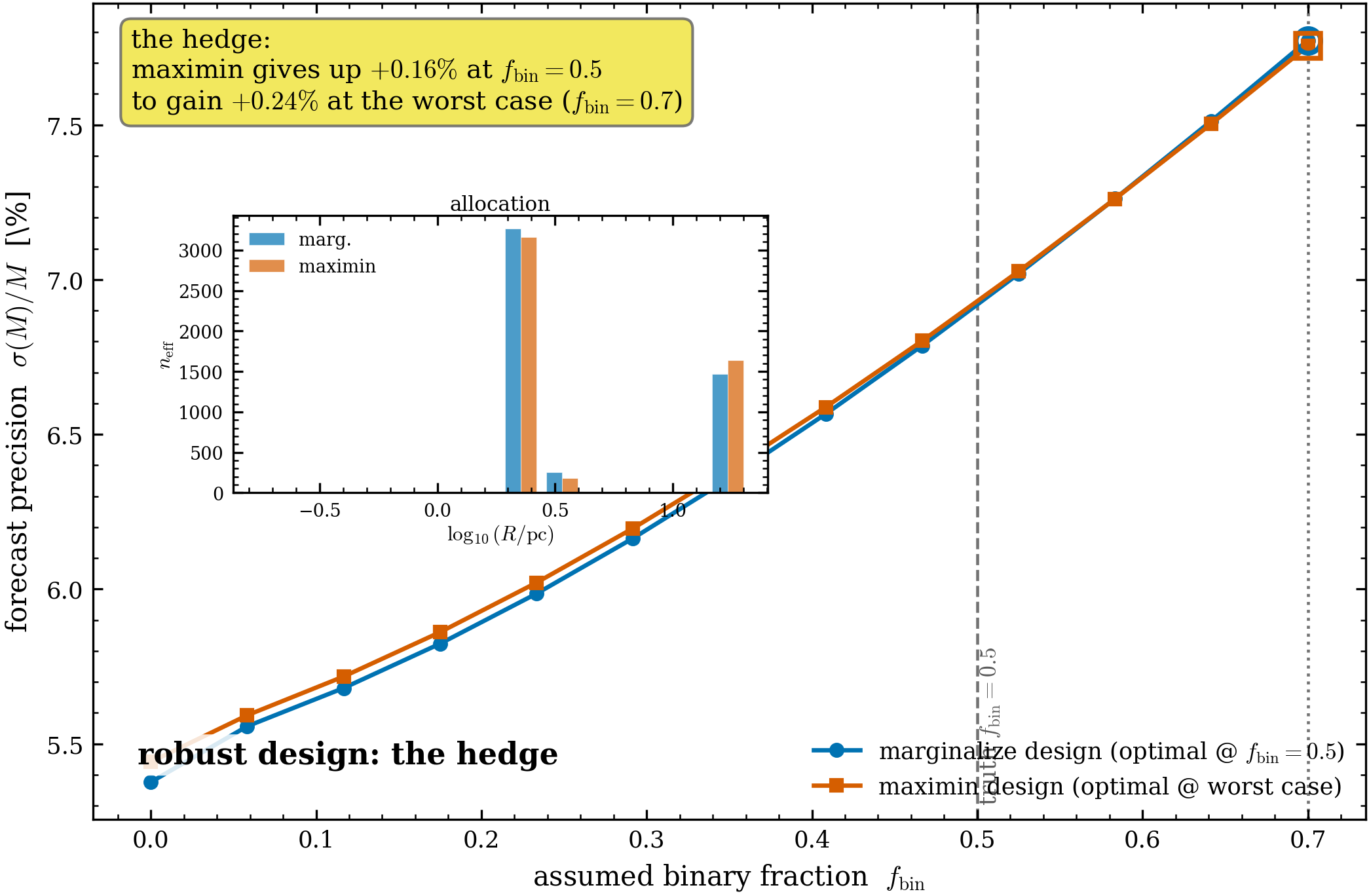
The robustness hedge is nearly free — and nearly pointless. Forecast vs the assumed binary fraction for the marginalize design (blue, optimal at the truth ) and the maximin design (vermilion, optimal at the worst case ). The two curves nearly coincide: is monotone in , so the marginalize design is already near-maximin-robust. The callout quantifies the hedge; the inset shows the two per-bin allocations barely differ. An honest near-null.
The sweep: the bias is catastrophic where binaries dominate
The fiducial operating point () is one slice through a continuum. Sweeping the system mass — which sets while stays fixed — traces the bias across contamination regimes, and it is the regime-of-validity map that turns a single number into a story.
The binary-blind-fit bias runs from (massive, hot clusters where binaries are a minor perturbation) to (low-mass, cold clusters where the pedestal swamps the cluster heat). Across the entire sweep the binary-aware fix holds the residual bias at . And the H2 precision-gain grows from at the fiducial point to where binaries dominate — so the thin operating-point margin is the floor, not the typical case. The colder the cluster, the more the binary-blind design lies, and the more the binary-aware design is worth.
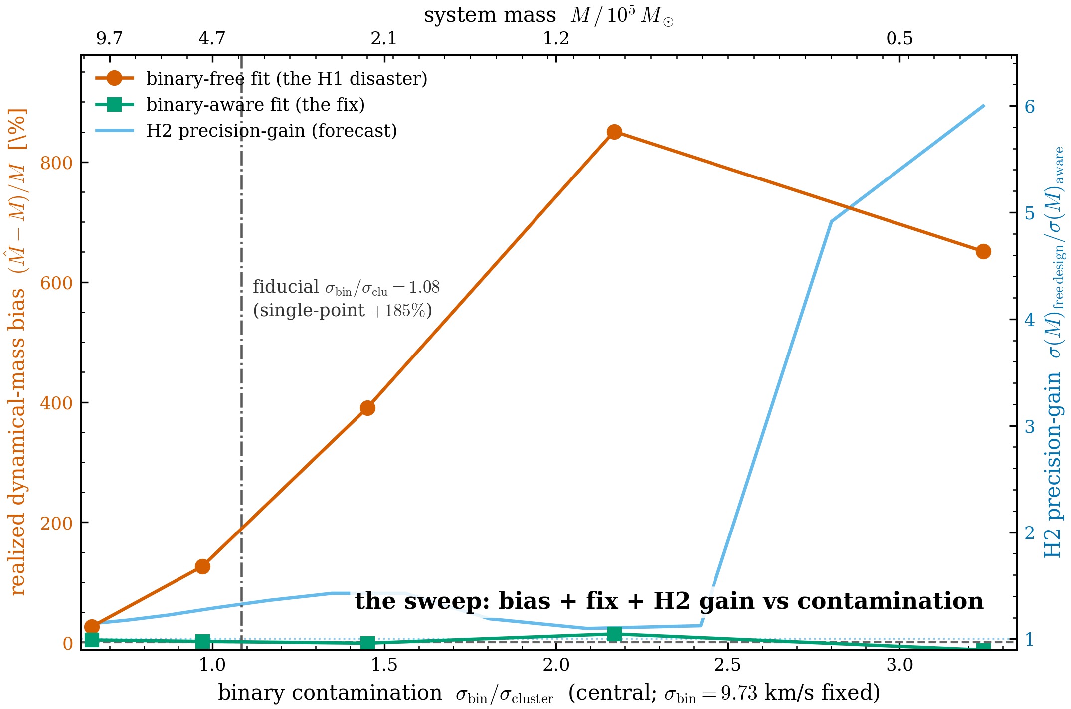
Bias, fix, and OED payoff across the contamination ratio. Left axis vs (top axis: system mass): the binary-blind-fit realized -bias (vermilion) rises from to as binaries come to dominate the cold outskirts of lower-mass clusters; the binary-aware-fit residual (green) stays flat at — the fix holds everywhere. Right axis: the H2 precision-gain (sky) grows from to . The fiducial operating point (the single-point headline) is marked.
Validating a pre-data calculation: two gates
A Fisher forecast is a promise — and this demo’s promise is the unusual one that a design will be biased. Both halves are checked.
Gate 1 — the gradients are correct (AD-vs-FD)
The load-bearing new derivatives are the Fisher block and the binary
-inflation term. We verify them against finite differences to
(Richardson where a fixed-step FD is truncation-limited), per gradient-validation. The
analytic column matches AD to
.
Gate 2 — the bias is real (cross-model Monte Carlo)
The bias claim is gated by a cross-model Monte Carlo: generate WITH Moe binaries, fit
WITHOUT. The mock is forward-model-consistent — the cluster mock is the fit model, so the
baseline is unbiased by construction and any bias is attributable to binaries
alone. Each draw places the design’s per-bin star counts directly, draws each star’s cluster
velocity from with from
project_dispersion at the truth, adds a flux-weighted Moe blend (from a build-once
pool rescaled to ) to the per-star
fraction, adds per-star , forms the
per-bin , and fits by MAP in the Gauss–Newton metric (honest
realized- weighting; unpopulated bins dropped, not floored). The H1 accept rule was fixed in advance: accept iff the mean
and the band does not
straddle that threshold. It is met by a wide margin (bias/forecast ; SEM 0.06). The
binary-aware fit’s accept rule — — is met by the
residual.
The pre-registration (locked before the Monte Carlo)
To keep the bias result honest, the hypotheses and accept/reject rules were locked before
the Monte Carlo ran, via research-workflow:discriminating-experiment-design. A reject on any
of them was defined in advance as a reportable finding, not a failure — and an H1 reject would
have descoped the whole arc.
Pre-registered hypotheses (locked 2026-06-19)
Hypothesis | Accept rule (fixed in advance) | Outcome |
|---|---|---|
H1 — the bias. Binary-blind design + binary-blind fit on contaminated data biases high beyond its own forecast. | , positive, SEM not straddling. | ACCEPT ( vs ; ) |
H0 — the rival. The binary-blind fit absorbs the pedestal into nuisances; stays unbiased. | . | rejected (the control is the unbiased case; is not) |
H2 — OED payoff. The binary-aware design beats the blind one under the binary-aware fit. | precision-gain . | ACCEPT ( at the operating point; in the sweep) |
H3 — non-obvious allocation. The binary-aware allocation is not a monotone rescaling of the blind one. | per-bin weight rank-order changes. | ACCEPT (drops 7.6 pc, concentrates 2.26 pc) |
Quantitative results
All numbers are from the gated CLI’s run-record (EFF-OM YMC operating point, , bins, cross-model MC 48 draws):
OED binary-robustness results
Quantity | Binary-blind (naive) | Binary-aware (fix) |
|---|---|---|
(cross-model MC, ) | ( bias) | (, within forecast) |
Claimed / honest | (claimed) | (honest, marginalized) |
bias / forecast ratio | (false confidence) | (calibrated) |
control bias | (unbiased — isolates the binaries) | — |
Recovered | — (not modelled) | (radial leverage) |
Prior-insensitivity ( looser prior) | — | moves (identifiable) |
H2 precision-gain (binary-aware design) | — | (fiducial); (binary-dominated) |
Maximin hedge over the marginalize design | — | (honest near-null) |
Sweep: -bias range across system mass | throughout |
What the optimum means: science implications
1. “Optimal” is only optimal under a correct model. The whole demo is a warning about the silent assumption inside every OED (and every analysis): the design that minimises your forecast variance under the wrong model can maximise your real error. A tighter forecast is not a better measurement — it is only a better measurement if the model is right. The binary-blind design’s was the most dangerous kind of number.
2. Population systematics are a design problem, not just an analysis problem. You cannot fix binaries purely after the fact if your survey spent its budget in the contaminated outskirts. The binary-aware design spends differently because it knows the pedestal exists — it earns the constraint from radial leverage at the telescope, not from a prior at the keyboard.
3. progenax can do this because it is differentiable end-to-end. Wiring a faithful Moe &
Di Stefano binary population into a Fisher design requires
through the binary kernel.
That is the throughline of the whole OED section: the same additive backbone that
targets anisotropy, mass, and
concentration here defends a measurement against a model error — it
extends OED from “what to measure” to “what to measure robustly.”
Current scope and planned extensions
How to run
# the cheap design + forecast + mechanism figure (no MC; CI-safe, ~1 min)
env -u VIRTUAL_ENV uv run --no-sync python scripts/demo_oed_binary.py

# the full result: cross-model MC (the H1 bias + headline figure) + maximin + sweep
PROGENAX_RUN_OED_BINARY=1 env -u VIRTUAL_ENV uv run --no-sync \
    python scripts/demo_oed_binary.py --run-mc --maximin --sweep \
    --outdir docs/website/60-science-demos/optimal-design/figures
The cheap default path computes the binary-blind design, its forecast , and the
mechanism figure, and exits 0. The env-gated cross-model Monte Carlo (the H1 bias, the
false-confidence figure) is @slow and out of CI — it is the gate
test_H1_naive_design_is_biased_beyond_forecast (and the binary-aware
test_fix_binary_aware_fit_is_unbiased) in tests/unit/test_demo_oed_binary.py, run with
PROGENAX_RUN_OED_BINARY=1. The figures and run-record land alongside this page.
References
The shared Fisher / Cramér–Rao / projection theory and its references are on the OED formalism page. The line-of-sight projection into is Binney & Mamon (1982); the Osipkov–Merritt anisotropy law is Merritt (1985); the EFF density profile is documented on the EFF profile theory page. The binary population — the –– engine behind — follows Moe & Di Stefano (2017), with ZAMS flux weights from Tout et al. (1996); the single-epoch binary-inflated dispersion machinery is the binary dynamical-mass demo (B12). The companion OED designs are anisotropy (where the proper motions belong), dynamical mass (how deep to survey), and concentration (where concentration information lives) — this page extends them to model robustness.
- Binney, J., & Mamon, G. A. (1982). M/L and velocity anisotropy from observations of spherical galaxies, or must M87 have a massive black hole? Monthly Notices of the Royal Astronomical Society, 200, 361–375. 10.1093/mnras/200.2.361
- Merritt, D. (1985). Spherical stellar systems with spheroidal velocity distributions. The Astronomical Journal, 90, 1027–1037. 10.1086/113810
- Moe, M., & Di Stefano, R. (2017). Mind your Ps and Qs: The interrelation between period (P) and mass-ratio (Q) distributions of binary stars. The Astrophysical Journal Supplement Series, 230, 15. 10.3847/1538-4365/aa6fb6
- Tout, C. A., Pols, O. R., Eggleton, P. P., & Han, Z. (1996). Zero-age main-sequence radii and luminosities as analytic functions of mass and metallicity. Monthly Notices of the Royal Astronomical Society, 281, 257. 10.1093/mnras/281.1.257