OED for anisotropy — where to spend telescope time on r_a (B14)
The optimiser discovers that proper motions belong in the outskirts — without being told the physics
This is the first worked example of optimal experimental design: given a fixed budget of stars, where on the sky and in which channel should you measure to pin one number — the cluster’s velocity anisotropy? The answer the optimiser returns, having been told none of the underlying physics, is the lesson: proper motions belong in the outskirts.
Reading paths
Already comfortable with Fisher OED? Skip to the physical question for the anisotropy science, or jump straight to the headline figure and Quantitative results.
Want the machinery first? Read the OED formalism page, then come back here.
The physical question: how do you measure orbital anisotropy?
Our target is the velocity anisotropy of a star cluster — the degree to which stellar orbits are radially or tangentially biased, captured by the Binney parameter Equation. We adopt the Osipkov–Merritt law Merritt, 1985,
isotropic in the core and increasingly radial outward, with a single knob: the anisotropy radius , the radius where . Measuring the cluster’s orbital structure is measuring .
Why does this matter physically? Anisotropy is a fossil of how a cluster formed and how it is being torn apart: violent relaxation, tidal stripping, and radial-orbit instability all leave their signature in . In dwarf-galaxy dynamics the same is the dominant nuisance in the mass–anisotropy degeneracy that limits dark-matter cusp-versus-core measurements. So is both a number worth measuring and a number that is notoriously hard to measure — which is what makes it a perfect OED target.
Why proper motions, and why the outskirts
The three sky channels — line-of-sight RV, radial PM, tangential PM — are the B&M82 projection Equation of one internal and . The key fact, derived there: in the isotropic limit the three channels are identical — the anisotropy lives only in their ratios. The tangential proper motion is the cleanest probe, , so as orbits turn radial it collapses while the other channels stay up. And because grows outward, the channels disagree most in the outskirts. A single profile cannot break the tie — a cold outer LOS profile can mean “low ” or “high .” Proper motions break it. Keep that picture in mind: it is the physics the optimiser is about to rediscover, having been told none of it.
Inputs and assumptions
The design optimises over a fixed budget of stars allocated across projected-radius bins 3 kinematic channels (36 cells). The science target is ; total mass and half-mass radius are nuisances carried with fractional priors. Everything is computed pre-data — no mock catalogue enters the optimisation loop (a 64-draw calibration ensemble afterwards is a gate, not part of the design).
Model inputs
Input | Meaning and role | Status (fiducial) |
|---|---|---|
Osipkov–Merritt anisotropy radius — the science target; . c-optimality minimises its marginal variance. | target (6.0 pc ; well inside OM validity ) | |
, | Total mass and Plummer half-mass radius — nuisances, profiled out; each carries a 30% fractional () prior (e.g. from integrated light, from photometry). | nuisances (, pc) with |
3 kinematic channels | RV (), PM radial (), PM tangential () — the design lever; each channel’s information content is set by the B&M82 kernels Equation. | fixed (the design allocates stars among them) |
, , | Distance converts the astrometric error to velocity; per-star errors enter the per-datum variance . At kpc the two channels are at deliberate error parity — neither trivially dominates. | fixed ( kpc; km/s; mas/yr km/s) |
completeness | Fixed realism, identical across channels: a smooth logistic faint-end roll-off ( in the core, outside, turnover ). Illustrative, not a real survey curve, and not a design knob here — promoting depth to a knob is the dynamical-mass example. | fixed (folds into the per-star blocks) |
bins, budget, optimiser | log-spaced bin centres ; budget (default 4000, swept for the frontier); multi-start Adam over the softmax simplex. | numerical choices |
units, |
| known / fixed |
The Fisher is built in the dimensionless metric Important, so is a fractional precision and the nuisance prior is fractional too (none on the target).
The method, specialised: c-optimality on the additive Fisher
This example pours the additive backbone
Equation straight into a c-optimal allocation. The per-star blocks
come from one jacrev of project_dispersion at the truth; the design enters
only through the softmax weights Equation, multiplied by the fixed completeness
. The headline criterion minimises the variance with profiled out:
We also run D () and A () as the contrast — see why c and D should disagree. Under the (through ) and degeneracies they put stars at different radii, which is the criterion-disagreement lesson made visible below.
Validating a pre-data calculation: the calibration ensemble
A Fisher forecast is a promise: “if you observe this way, your error bar will be this large.” A promise made before any data is only trustworthy if you check it, because the Cramér–Rao bound Equation is a local, Gaussian approximation — exact in the high-information limit, optimistic when the likelihood is curved or the estimator is biased.
So we close the loop once, as a gate (not inside the optimiser). We draw a 64-member ensemble of mock catalogues from the actual Osipkov–Merritt Plummer sampler, project each to the sky, bin it, and fit by maximum a posteriori (with the same fractional prior the design Fisher used). The realised scatter should match the Fisher prediction,
both sides being fractional variances in the metric. The tolerance is not a free knob: the Monte-Carlo error on a variance estimated from draws is , so the gate is a principled band, . The realised sits just below the Fisher’s 0.121 — the pre-data Fisher is mildly conservative (the binned-dispersion estimator loses a little information relative to the idealised per-star Fisher), and the two agree well inside the band. The promise holds.
Figures
The headline — PMs to the outskirts
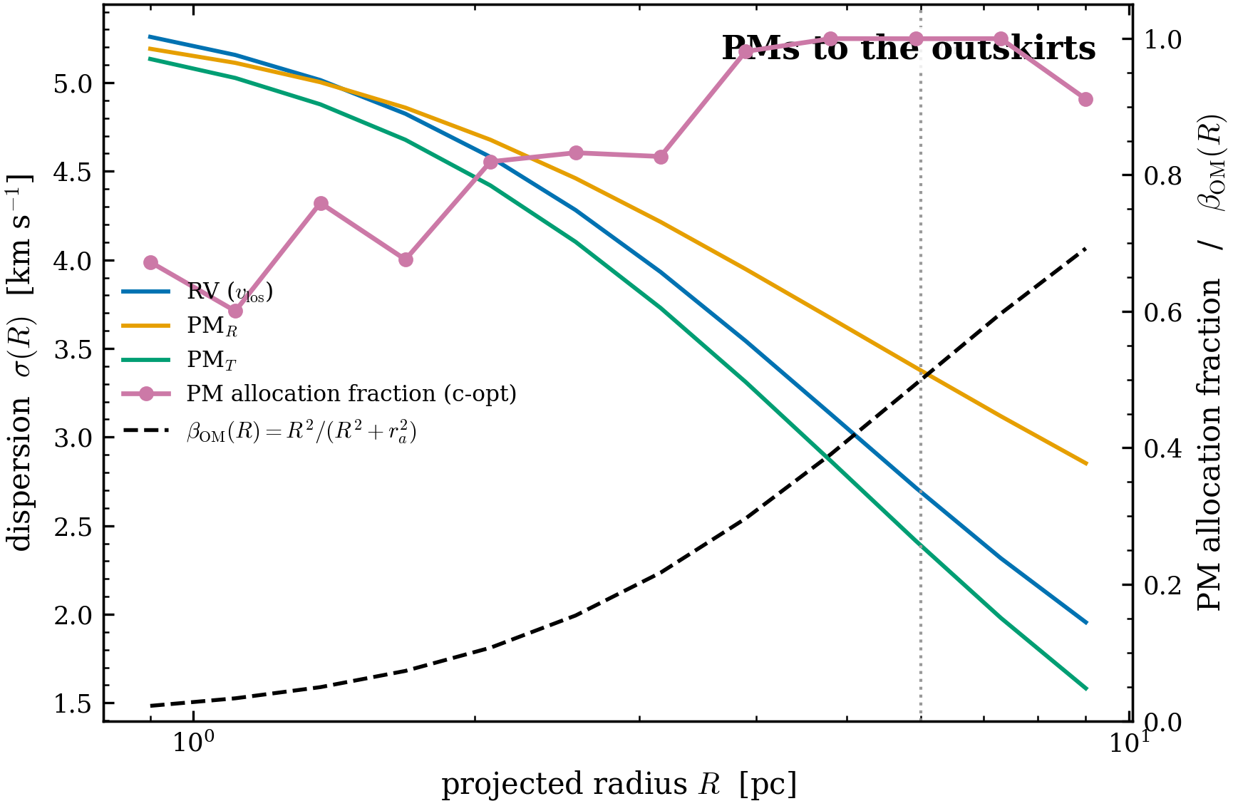
The c-optimal design tracks the OM anisotropy . Left axis: the three predicted dispersion channels , , (km/s) vs projected radius. Right axis: the c-optimal PM allocation fraction per bin (purple) plotted against (dashed). The design — told nothing about anisotropy — pushes the PM share from 0.73 in the core to 0.95 in the outskirts, following : proper motions go where the anisotropy signal is.
c vs D vs A — why the criteria disagree
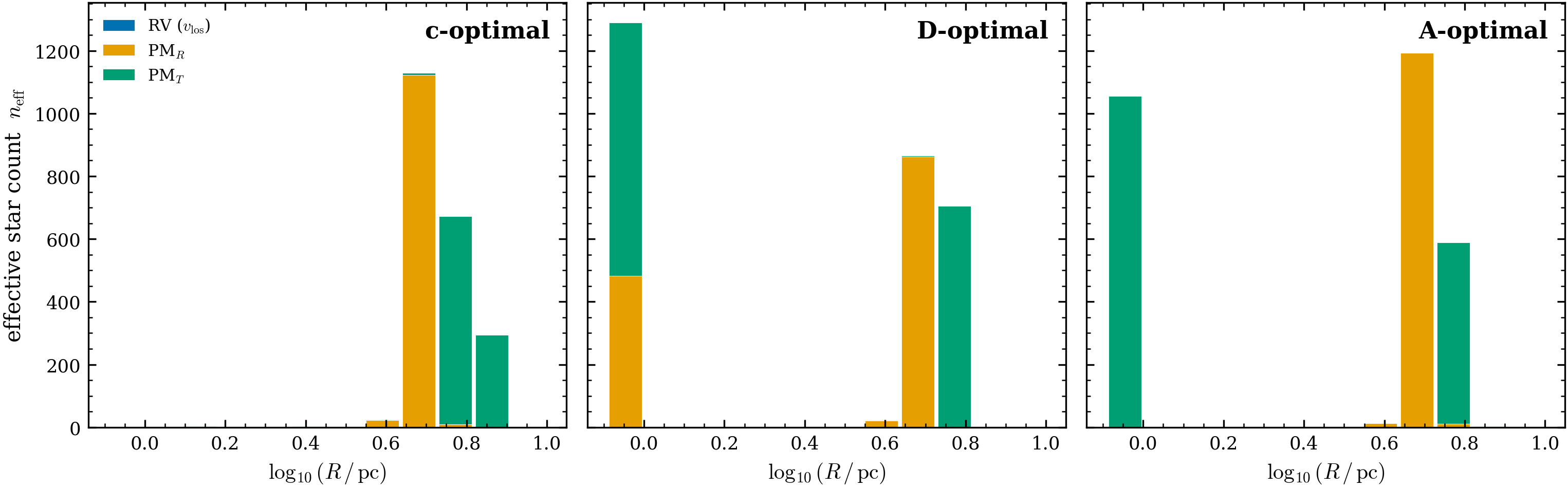
The c-, D-, and A-optimal allocations differ. Each panel stacks the effective star count per channel over radius for one criterion. The c-design (targeting alone) loads the PM channels in the outskirts hardest; the D- and A-designs, which must constrain and too, also load the core, where the density and overall normalisation are best pinned. Different objectives genuinely want stars at different radii — the disagreement is shown, not asserted.
The precision frontier — fewer stars at equal precision
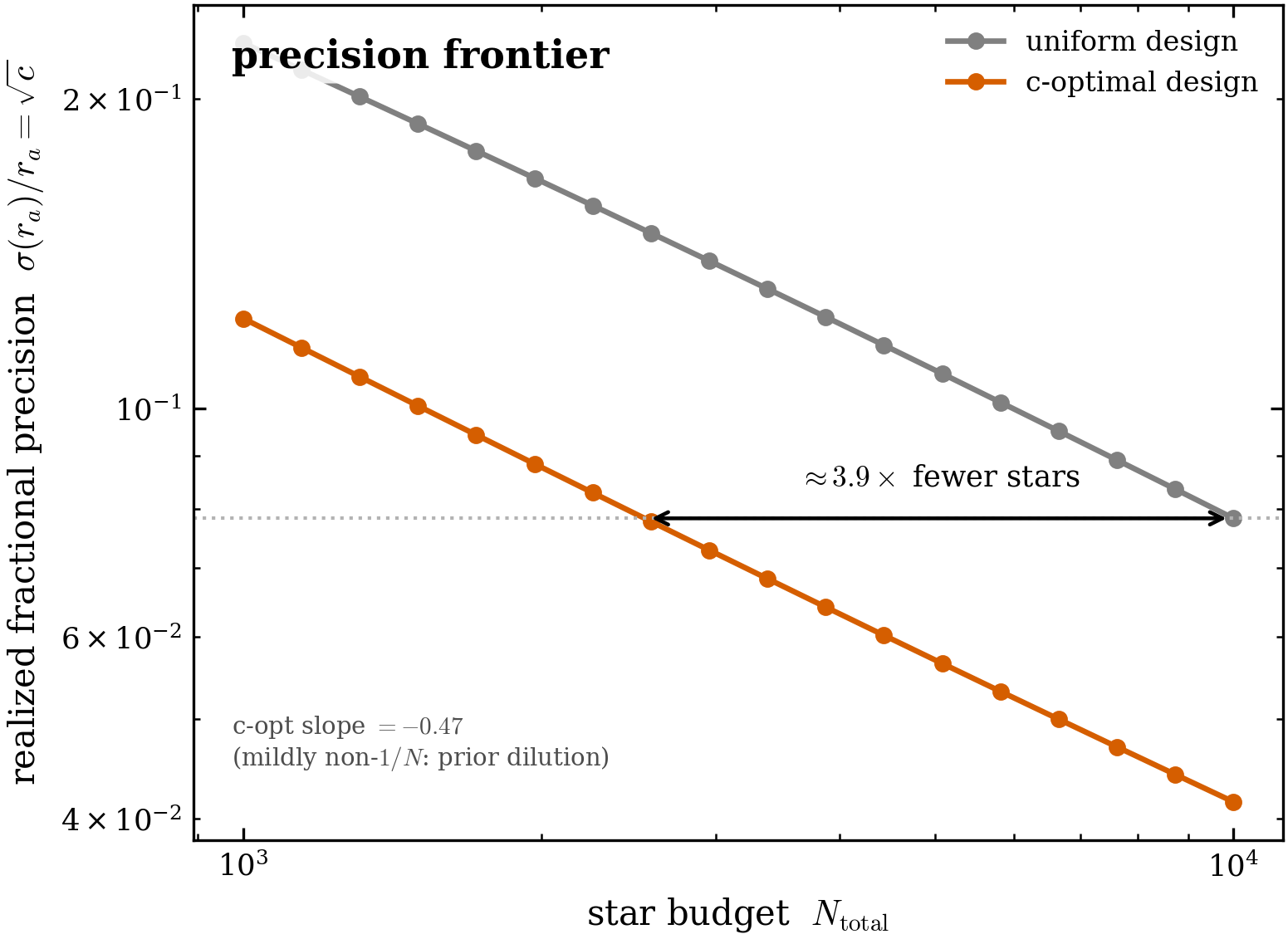
The c-optimal design reaches equal precision with fewer stars. Realized fractional precision vs star budget , recomputed (not extrapolated) for the uniform and c-optimal designs. The horizontal arrow is the equal-precision star factor at the reference precision. The curves are mildly non- because the fixed nuisance prior dilutes as grows (the c-opt slope departs slightly from ) — the honest, real frontier rather than an idealised line.
Calibration — the pre-data Fisher is trustworthy
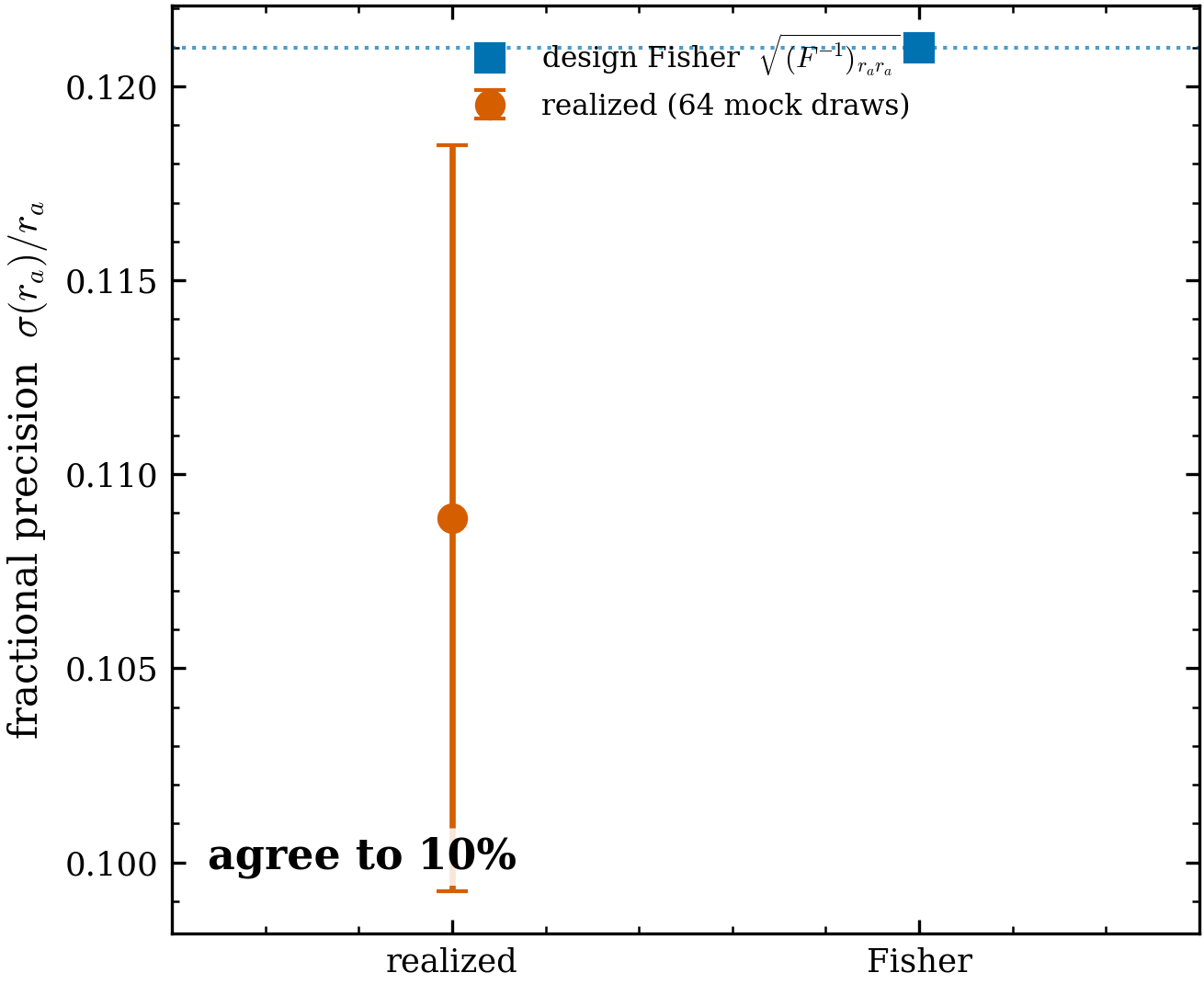
A 64-draw mock ensemble confirms the design Fisher predicts the realized scatter. The calibration is run at the uniform design (so the Fisher value here, 0.121, is the uniform precision — not the c-optimal 0.063); this suffices because the per-star Fisher blocks are design-independent, so validating the Fisher machinery at one design transitively validates it at the c-optimal design built from the same blocks. The realized fractional precision (orange, with its Monte-Carlo error band from 64 draws) sits at 0.109, just below the Fisher-predicted 0.121 (blue): the pre-data Fisher is mildly conservative, and the two agree within the MC error. This is the gate that makes the pre-data design trustworthy.
Optimiser convergence
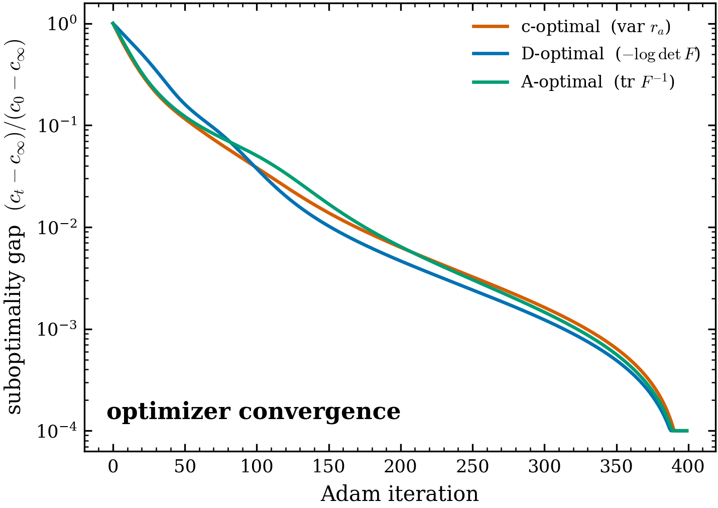
All three alphabet-optimality objectives converge cleanly. Each curve is the best-start suboptimality gap vs Adam iteration, normalised to the initial gap (the c, D, A objectives live on different scales and signs, so the normalised gap is the like-for-like view). Every objective descends monotonically to its converged design.
Quantitative results
All numbers are from the gated CLI’s run-record (--full, 64-draw calibration,
):
OED anisotropy results
Quantity | Result |
|---|---|
Equal-precision star factor (c-design vs uniform, fixed ) | fewer stars ( on the swept frontier) |
, uniform c-optimal (at fixed ) | |
PM allocation fraction, inner-half outer-half (c-design) | (PMs favoured outward) |
Calibration: realized vs Fisher | 0.109 (realized) vs 0.121 (Fisher) — variance-space dev, gate |
c-criterion : uniform / c-opt / D-opt / A-opt | (c-design lowest on its own objective) |
The equal-precision factor is exact at fixed (the fixed nuisance prior cancels in the ratio, because when the prior is held fixed); the “ fewer stars” gloss on the frontier is the same physics read off the swept budget curve, where the prior no longer cancels and the slope departs mildly from .
What the optimum means: science implications
The is not a free lunch — it is the optimiser discovering the physics of where information lives, and it generalises well beyond this mock.
1. Information is localised — in space and in channel. Anisotropy grows outward, and the tangential-PM sensitivity to grows with it. So the value of a star for measuring depends sharply on where it sits and how you measure it. OED makes that quantitative instead of intuitive: the headline figure shows the optimiser routing PM stars to exactly the radii where is turning over.
2. Proper motions break the mass–anisotropy degeneracy where it bites. A line-of-sight dispersion profile alone is degenerate — recall Equation: a cold outer can mean low or high . The two PM channels carry different -weightings Equation, so they lift the degeneracy — and the OED tells you where the lift is largest: the outskirts. The result — RV in the core, PM in the outskirts — is the observing strategy this degeneracy demands, derived from first principles. That is directly actionable for real Gaia-PM + spectroscopic campaigns on globular clusters and dwarf spheroidals.
3. Design for your target, not for “everything.” The c-vs-D-vs-A divergence is the deepest lesson. If your science is one number — anisotropy as a probe of a dark-matter cusp/core, an IMBH’s kinematic signature, a cluster’s tidal state — a design that minimises the joint ellipsoid (D) wastes stars tightening nuisances. c-optimality can buy a multiplicative factor in the precision you actually care about.
4. The honest caveat is itself a research direction. The optimum is optimal for the
assumed OM-Plummer model. That model-dependence is the central limitation of all OED —
and it points straight at the most valuable extension: robust and
model-discriminating design (see the section’s capability map), which
progenax is unusually well-placed to do because it ships more than one differentiable
forward model for the same observable.
Current scope and planned extensions
How to run
# quick (12-draw calibration, ~1 min)
env -u VIRTUAL_ENV uv run --no-sync python scripts/demo_oed.py

# publication-grade (64-draw calibration, ~4 min) — regenerates the figures here
env -u VIRTUAL_ENV uv run --no-sync python scripts/demo_oed.py --full
The CLI is gated (exit 0 only if the headline factor, PM-outskirts trend, and calibration all pass) and writes a JSON run-record alongside the five figures.
References
The shared Fisher / Cramér–Rao / projection theory and its references are on
the OED formalism page. The Osipkov–Merritt anisotropy law is
Merritt (1985); the line-of-sight projection into ,
, is Binney & Mamon (1982, MNRAS 200, 361). The
differentiable project_dispersion forward model is documented on the
velocity-DF kinematics pages; the
anisotropy recovery counterpart is the anisotropy demo (B6), and
B8 introduces the same sky-projection helper.
- Merritt, D. (1985). Spherical stellar systems with spheroidal velocity distributions. The Astronomical Journal, 90, 1027–1037. 10.1086/113810