OED for concentration — where to spend telescope time on W₀ (Stage 3)
The optimiser sends the proper motions to the CORE to measure concentration — the mirror image of the anisotropy design
OED for concentration — where to spend telescope time on (Stage 3)
You have a cluster and a star budget, and you want to know how centrally concentrated it is. The anisotropy design asked where on the sky and in which channel to measure to pin the orbital anisotropy ; the dynamical-mass design asked how deep to survey to weigh the cluster. This page asks the same kind of question for a third target — the cluster’s concentration — and the optimiser returns an answer that is the mirror image of the anisotropy result. Anisotropy wanted the outskirts; concentration wants the core. Same machinery, opposite strategy, and the contrast is the lesson.
Reading paths
Already comfortable with Fisher OED? Skip to the physical question for the concentration science, or jump straight to the headline figure and Quantitative results.
Want the machinery first? Read the OED formalism page, then come back here.
Why does this demo exist at all? It closes the loop on the W₀-differentiability work — see why this arc exists.
Why this arc exists: closing the W₀-differentiability loop
A short piece of history makes the rest of the page land. The forward models that turn a
cluster’s structure into observable dispersions — the Osipkov–Merritt Jeans projection
project_dispersion and the exact Michie second moment df_moment_dispersion — were made
differentiable in the concentration by two pieces of internal work: a
PCHIP interpolation of the King/Michie equilibrium-solver tables and a
lock on the df_moment path. Those changes made
exist and be smooth.
But they were validated only at the gradient-audit level — an automatic-versus-finite-difference check that the derivative is numerically correct (98 entry points, 0 hazards). They were never exercised through an actual Fisher / OED inference that treats as a parameter. The stated goal of that whole line of work — “-differentiable for OED/Fisher” — had an open loop. This demo closes it: it builds the design Fisher with in the parameter vector, optimises an observing strategy for it, and confirms the forecast against real mock catalogues. It is the end-to-end use of the capability those ADRs promised.
The physical question: how do you measure concentration?
Our target is the concentration of a star cluster — how steeply its density climbs from the tidal boundary to the centre. For the King (1966) lowered-isothermal family the concentration is governed by a single dimensionless number, the central potential depth (documented on the King profile theory page): a small is a diffuse, weakly-bound cluster; a large is a deep, centrally-peaked one with an extended outer envelope. sets the King concentration — the ratio of tidal to core radius — so measuring how concentrated a cluster is means measuring .
Why does this matter physically? Concentration is a dynamical clock and a structural fingerprint: it tracks core collapse, two-body relaxation, and the cluster’s tidal history, and it is the first parameter any structural model of a globular cluster or a dwarf must pin. It is usually read off the surface-density / star-count profile — that is the count-channel recovery demo (B11). Here we ask the complementary question: what does the kinematic dataset say, and where in it does the concentration information live?
Why concentration is a core probe — the physical intuition
The key fact, which the optimiser is about to rediscover unaided: concentration is an isotropic, central property. Changing rescales the depth of the potential well, and its strongest observable fingerprint is the velocity dispersion contrast between the deep core and the cold outskirts. A more concentrated cluster has a hotter, more sharply peaked in the core, falling to a colder envelope; a diffuse one is flatter. The core is where the dispersion is highest and the projected density is greatest, so it is where a fixed number of stars pins that contrast most tightly. This is the opposite of anisotropy, which is zero in the core by construction () and only grows outward — so the anisotropy signal lives in the outskirts. Hold that contrast in mind: concentration → core, anisotropy → outskirts. It is the physics behind the headline figure.
Inputs and assumptions
The design optimises over a fixed budget of stars allocated across projected-radius bins 3 kinematic channels (36 cells). The science target is ; the anisotropy radius is a co-determined kinematic parameter and the total mass is a nuisance carried with a fractional prior. Everything is computed pre-data — no mock catalogue enters the optimisation loop (a real-star calibration ensemble afterwards is a gate, not part of the design).
Model inputs
Input | Meaning and role | Status (fiducial) |
|---|---|---|
King/Michie central potential depth — the science target; sets the concentration . c-optimality minimises its marginal variance. | target (; index 0 of ) | |
Osipkov–Merritt anisotropy radius — a co-determined kinematic parameter (no external prior; constrained by the RV-vs-PM split alone). The same is the OM radius passed to | free (; index 1) | |
Total mass — the only nuisance with an external constraint (integrated light ); carries a 30% fractional () prior. | nuisance (; index 2) with | |
profile model | King (headline OM-King) and Michie, both projected under Osipkov–Merritt — they differ only in the density → map (see the modelling choice). | two models compared |
3 kinematic channels | RV (), PM radial (), PM tangential () — the design lever; each channel’s information set by the B&M82 kernels Equation. | fixed (the design allocates stars among them) |
, , | Distance converts the astrometric error to velocity; per-star errors enter the per-datum variance . At kpc the two channels are at deliberate error parity — neither trivially dominates per component. | fixed ( kpc; km/s; mas/yr km/s) |
completeness | Fixed realism, identical across channels: a smooth logistic faint-end roll-off ( in the core, outside, turnover ). Illustrative, not a real survey curve, and not a design knob here — promoting depth to a knob is the dynamical-mass example. | fixed (folds into the per-star blocks) |
bins, budget, optimiser | log-spaced bin centres (every bin inside both models’ , so all are bound); budget (the King calibration operating point); multi-start Adam over the softmax simplex. | numerical choices |
units, |
| known / fixed |
The Fisher is built in the dimensionless metric Important, so is a fractional precision and the nuisance prior is fractional too — none on the target , none on , only on . That the data alone (three velocity channels 12 radial bins) keep the 2-block positive-definite — so no prior on or is needed for a well-posed inverse — is a measured property of this design, not an assumption (it is checked across random designs in the test suite).
The modelling choice: OM-King and OM-on-Michie-density
Two facts about the forward model set up the whole demo, and stating them plainly is the honest way to read the result:
project_dispersionis Osipkov–Merritt only. It imposes Equation on whatever density it is handed — it does not read a profile’s own intrinsic anisotropy. So both models here are projected under the same OM anisotropy law; they differ only in the density profile, and hence in the concentration-dependent map . King is isotropic in density (OM is layered on top); Michie carries its own native anisotropy in its density shape, but it is still projected under OM. The headline is OM-King; Michie is added to exercise the native path explicitly and to test that the qualitative answer is robust to the density model.The calibration’s sampler equals the Fisher model. The real-star gate (below) must draw stars from the exact distribution
project_dispersionprojects — “that density under OM” — or it would validate a mismatched model. So the OM particle sampler is assembled to be self-consistent with the Fisher forward model: for King via the Engine BMultiComponentCluster.from_density_profilespath (a single-component King density in its own shared- potential with an Eddington/OM DF, documented on the Engine B validation page); for Michie via the generic Eddington inversion (, Merritt 1985 augmented density) on the Michie density, since Engine B does not ingestMichieProfile. In both cases sampler Fisher-model, which is what makes the calibration a real test rather than a tautology. (Deliberately we do not useMichieVelocityDF’s native — that would mismatch the OM projection and bias the gate.)
The method, specialised: c-optimality on the additive Fisher
This example pours the additive backbone
Equation straight into a c-optimal allocation, exactly as the
anisotropy design does — only the target index changes. The per-star blocks come
from one jacrev of project_dispersion at the truth (reverse-mode by policy — the
King/Michie equilibrium solvers hit a custom_vjp ODE with no forward-mode rule); the
design enters only through the softmax weights Equation, multiplied by the fixed
completeness . The headline criterion minimises the variance with and
profiled out:
We also run D () and A () as the contrast — see why c and D should disagree. Because the whole Fisher is additive and design-linear, the expensive projection is never re-differentiated inside the optimiser loop: one Jacobian, then invert a read one element.
Validating a pre-data calculation: two gates
A Fisher forecast is a promise — “if you observe this way, your error bar will be this large” — and a promise made before any data is only trustworthy if you check it, because the Cramér–Rao bound Equation is a local, Gaussian approximation. This demo checks it twice.
Gate 1 — the gradient is correct (AD-vs-FD on )
The load-bearing differentiability claim is the column of the Jacobian. We verify it against finite differences at every radial bin. For OM-King the automatic and finite-difference gradients agree to better than 10-3 across all bins. For OM-Michie the inner bins () agree to the same 10-3 with a fixed step, but at mid-to-outer radii the proximity of Michie’s truncation makes a fixed-step finite difference an unreliable proxy — the function has high curvature there (the truncation-curvature signature). So those bins are gated by Richardson finite differences instead: we confirm that as the step , the finite difference converges toward the automatic gradient. It does, to , at every bin — the automatic gradient is correct everywhere; the mid-radius values are pure truncation, not a code defect.
Gate 2 — the forecast is calibrated (real-star King calibration)
A Fisher forecast must predict the realized scatter of the estimator. We close the loop with a real-star ensemble: for the King model we draw independent mock catalogues from the OM sampler (which equals the Fisher forward model), project each to the sky, bin it by projected radius, subsample the design counts, add per-star measurement error, and fit by maximum a posteriori in the Gauss–Newton metric (a Levenberg–Marquardt MAP fit, started at the truth). The realised fractional scatter should match the Fisher prediction,
both sides being fractional variances in the metric. The tolerance is not a free knob: the Monte-Carlo error on a variance estimated from draws is , so the gate is a principled band. The realised / Fisher variance ratio for King is 0.976 — comfortably inside the band, with no significant bias. The promise holds.
The headline result: concentration wants the core
The pre-registered hypothesis (H1) was: ’s optimal allocation differs from ’s — more core/intermediate weight, more channel-balanced, with only a modest outward pull. The result splits cleanly into a confirmed radial prediction and a refuted channel sub-prediction. Reporting both honestly — the hit and the miss — is the point; a wrong pre-registered sub-prediction is a genuine finding, not a failure.
RADIAL: confirmed — the mirror image of the anisotropy design
The c-optimal design puts of its stars in the core half of the radial range (King; Michie). The Stage-1 anisotropy design put in the outskirts. They are mirror images, and the physical reason is exactly the intuition above: concentration is an isotropic, central property imprinted where the dispersion is highest and the density greatest (the core), while anisotropy lives in 's outward growth (the outskirts). The optimiser was told none of this — it discovered where the concentration information lives.
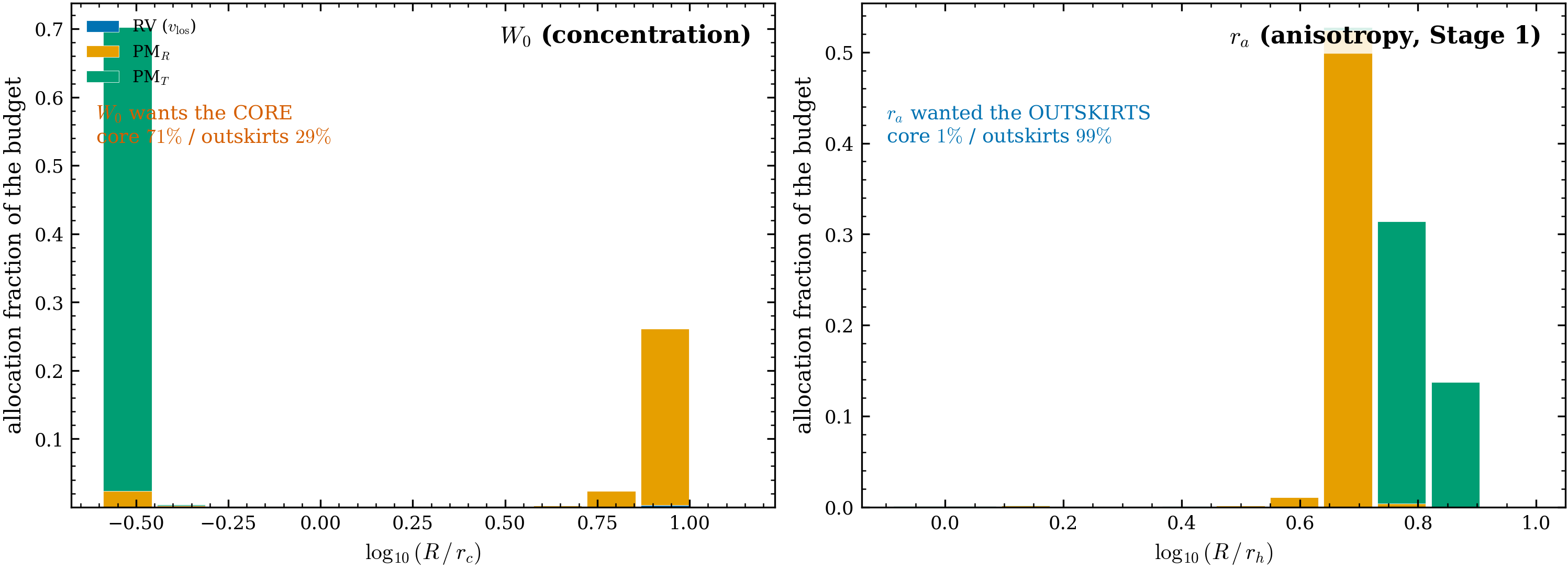
Concentration wants the core; anisotropy wanted the outskirts — the same machinery, opposite strategies. Left: the c-optimal radial allocation (King), stacked by channel (RV, PM, PM), as a fraction of the budget — core-heavy ( in the inner half). Right: the Stage-1 c-optimal allocation — outskirts-heavy ( in the outer half). Each panel is normalised to its own budget so the shape is compared (the grid is in ; the grid is in ). The mirror image is the pre-registered radial prediction H1, confirmed.
CHANNEL: refuted — concentration is strongly PM-dominated
H1 also predicted that would be more channel-balanced than (RV pulling more of its weight). It is not. The c-optimal design is strongly proper-motion dominated — RV carries only of the King budget. The reason is structural and the same one the anisotropy page documents: at the assumed RV/PM error parity, a proper-motion star delivers two information-bearing components (PM and PM) for one measurement, a 2-for-1 efficiency that the optimiser exploits almost everywhere. The error parity is per component, so PM wins on count. This sub-prediction was wrong, and we say so: it is a null result reported with integrity, and it sharpens the real lesson — the radial contrast (core vs outskirts) is the robust discriminator between the two targets, not the channel mix.
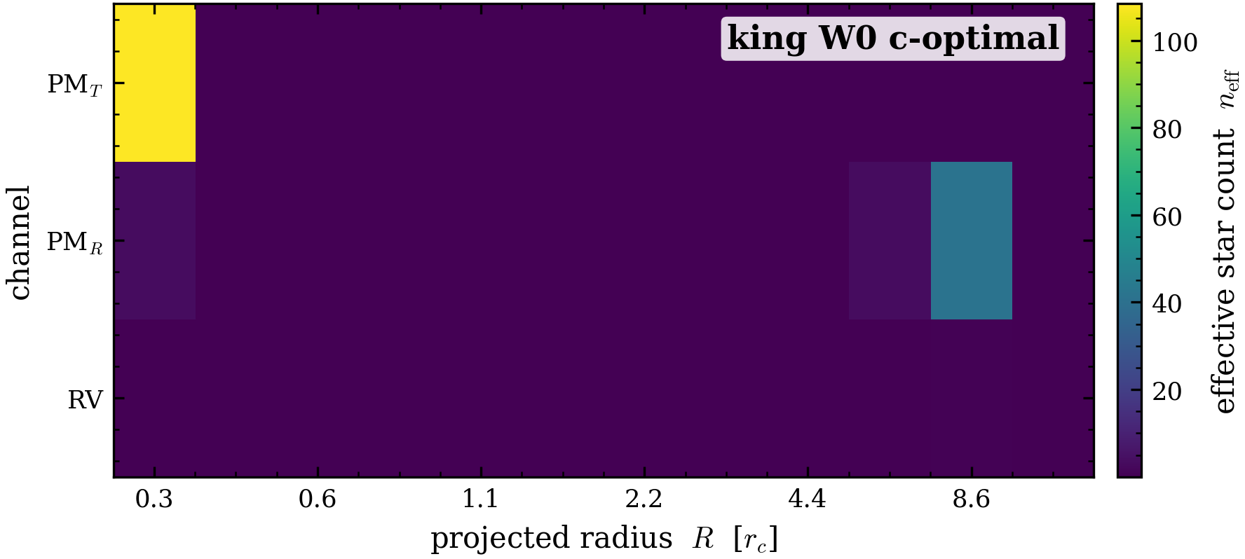
The King c-optimal allocation, resolved in both axes. Effective star count per (channel projected-radius) cell: rows are the three velocity channels (RV, PM, PM), columns the log-spaced on-sky radii. The budget piles into the core bins (left columns) and into the two proper-motion rows — the two-axis view of “concentration wants PMs in the core.” The RV row is nearly empty, the 2-for-1 PM efficiency made visible.
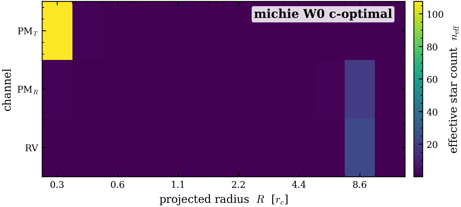
The Michie c-optimal allocation — the same qualitative answer. As The King c-optimal allocation, resolved in both axes. Effective star count per (channel projected-radius) cell: rows are the three velocity channels (RV, PM, PM), columns the log-spaced on-sky radii. The budget piles into the core bins (left columns) and into the two proper-motion rows — the two-axis view of “concentration wants PMs in the core.” The RV row is nearly empty, the 2-for-1 PM efficiency made visible., for the Michie density. The core-plus-PM structure is robust to the density model; Michie wants modestly more RV and a slightly more outward balance (see King vs Michie), but the headline strategy is unchanged.
The precision gain and the criterion contrast
How much does designing for concentration buy you? At fixed budget the King c-optimal design reaches a fractional precision , versus 0.104 for a uniform design — a gain in precision, equivalent to reaching the same error bar with fewer stars (the precision gain squared, since variance scales as when the prior is held fixed). The Michie design improves , a gain. As in the anisotropy example, the c-, D-, and A-optimal designs genuinely differ — the c-design, which only cares about , beats the others on its objective and would waste stars if it chased the whole ellipsoid.
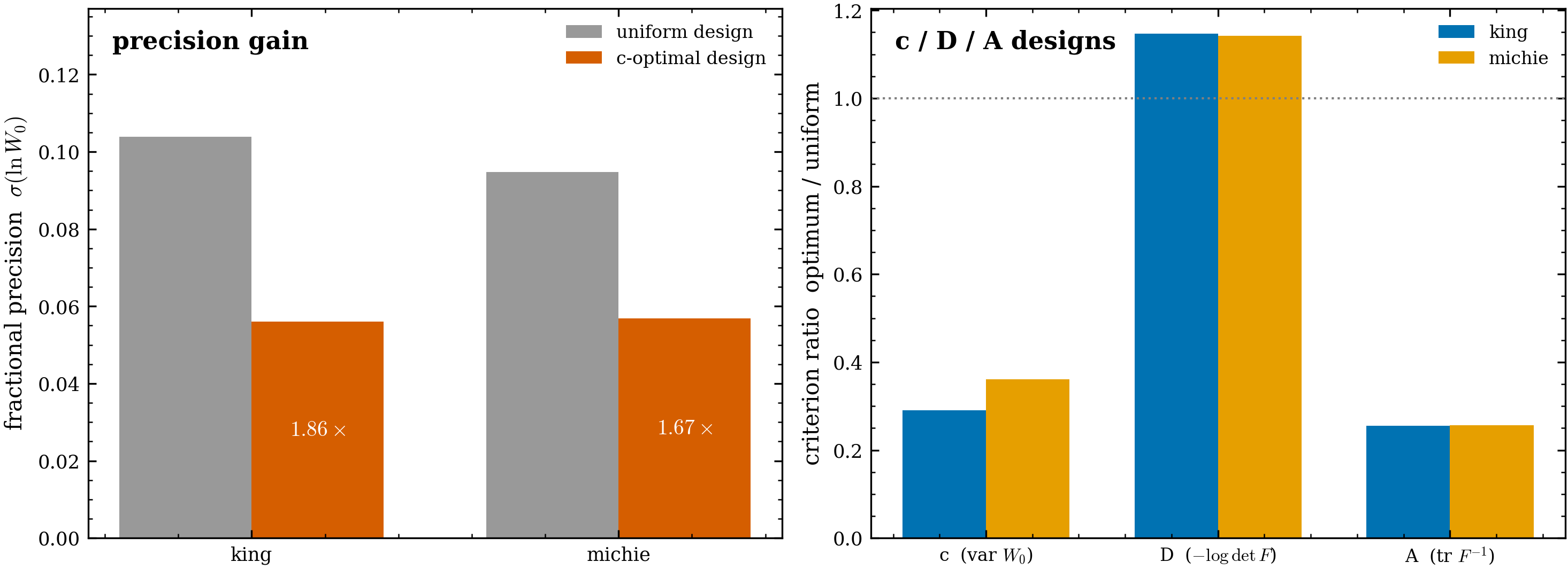
The precision gain and the c/D/A criterion contrast, King vs Michie. Left: the fractional precision for the uniform vs the c-optimal design (the gain factor is annotated on each c-optimal bar) — (King), (Michie). Right: each of the c/D/A optima as a ratio to its own uniform-design value (so all three are dimensionless “fraction of the uniform criterion”; is better), King vs Michie. The three alphabet-optimality designs are genuinely different objectives on the same .
The broken degeneracy: concentration is separable from anisotropy
The deepest science payoff is that this design breaks the degeneracy — it measures concentration and anisotropy independently. The Fisher correlation at the c-optimal design,
is the covariance off-diagonal normalised to : would mean the two are nearly degenerate (you cannot tell them apart), that the design measures them cleanly. We find for King and -0.12 for Michie — both far from . Concentration is cleanly separable from anisotropy in this kinematic design space, which is exactly what makes a -targeted observing strategy worth computing: the core-PM stars that pin are not the same stars that pin , and the design knows it.
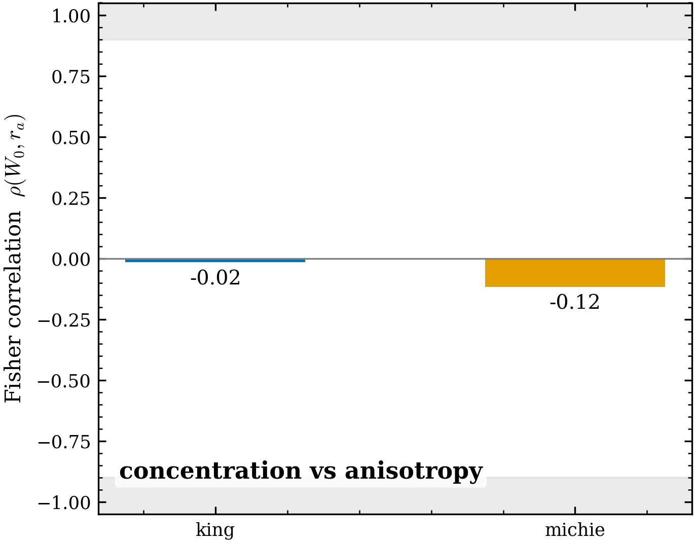
Concentration is separable from anisotropy. The Fisher correlation at the c-optimal design, King vs Michie. Both bars sit near zero (-0.02 King, -0.12 Michie), far from the shaded “near-degenerate” band: the design pins almost independently of . (A small negative is the residual, broken degeneracy — not a problem, but the quantitative statement of how well it is broken.)
King vs Michie: is the answer robust to the density model?
Yes, qualitatively. The headline — core plus proper motions — is the same for both density models, and the precision gains ( vs ) and core fractions ( vs ) are close. The differences are second-order and model-dependent: Michie wants modestly more of the RV channel ( vs ) and a slightly more outward balance, because its native-anisotropy density shape moves the contrast a little. The robust, model-independent statement is the one to take away: measure concentration in the core, with proper motions. The RV fraction and the fine radial balance are where the model choice shows up.
Quantitative results
All numbers are from the gated CLI’s run-record (, bins, the King calibration operating point):
OED concentration results
Quantity | King | Michie |
|---|---|---|
, uniform c-optimal (fixed ) | ||
Precision gain (c-design vs uniform) | ( fewer stars) | |
Core fraction (inner-half share, c-design) | 0.71 | |
Channel split RV / PM (c-design) | (PM-dominated) | |
Fisher correlation at c-optimal | -0.02 (separable) | -0.12 (separable) |
Contrast: Stage-1 c-optimal radial split | outskirts | — |
Real-star calibration (realized / Fisher) | (within band) | not run (OOM; see caveat) |
The precision gain is exact at fixed (the fixed nuisance prior cancels in the ratio, because when the prior is held fixed); the “ fewer stars” gloss is the same physics read as a star factor ().
What the optimum means: science implications
The result is the optimiser discovering where concentration information lives, and it generalises well beyond this mock.
1. The observing strategy is the opposite of an anisotropy campaign. To measure concentration, put the proper-motion budget in the core; to measure anisotropy, put it in the outskirts. Same instrument, same channels, opposite radial allocation — because concentration is a central, isotropic property and anisotropy is an outer, radial one. That is directly actionable: a Gaia-PM + spectroscopic campaign optimised for should not reuse an anisotropy campaign’s footprint, and OED tells you so quantitatively.
2. Concentration and anisotropy are independently measurable. The near-zero Equation means the kinematic dataset can pin both without one contaminating the other — the core-PM stars that constrain are not the outskirts-PM stars that constrain . A joint structural+orbital fit is well-posed in this design space, and the design is what makes it so.
3. Differentiable OED is a general tool. This is the third distinct science target
(, , now ) run through the same additive-Fisher machinery, each with a
different physical answer the optimiser found unaided. Because progenax’s forward models
are differentiable, is
computable for essentially any cluster-science parameter — which is the throughline of
the whole OED section.
4. The honest caveat is itself a research direction. The optimum is optimal for the
assumed OM-King/Michie model, and it rides the Jeans path, not the exact-moment one. That
model-dependence is the central limitation of all OED, and it points at the same valuable
extensions the sibling pages flag: robust, Bayesian, and model-discriminating
(T-optimal) design — for which progenax is well-placed because it ships more than one
differentiable forward model for the same observable.
Current scope and planned extensions
How to run
# the cheap design + figures (one jacrev per model + 3x3 linalg; ~1 min)
env -u VIRTUAL_ENV uv run --no-sync python scripts/demo_oed_concentration.py

# regenerate into the docs figure directory
env -u VIRTUAL_ENV uv run --no-sync python scripts/demo_oed_concentration.py \
    --outdir docs/website/60-science-demos/optimal-design/figures
The CLI computes only the cheap parts — one jacrev per model at the truth, the c/D/A
-linear-algebra optimisation, the H1 radial/channel split contrasted with Stage-1,
and the five figures — and writes a JSON run-record alongside them. The expensive real-star
King calibration is the env-gated @slow test
test_W0_fisher_calibration_matches_realized_scatter; the King ratio of 0.976 quoted
here is cited from that gate, not re-run in the CLI (the Michie MAP-MC is intentionally never
run — see the caveat).
References
The shared Fisher / Cramér–Rao / projection theory and its references are on the OED formalism page. The King (1966) lowered-isothermal model and its parameter are documented on the King profile theory page; the Michie–King anisotropic model on the Michie–King theory page; the Engine B Eddington/OM sampler on the Engine B validation page. The Osipkov–Merritt anisotropy law is Merritt (1985); the line-of-sight projection into , , is Binney & Mamon (1982). The count-channel concentration recovery — the complementary way to measure , from star counts rather than kinematics — is the King-concentration demo (B11); the companion OED designs are anisotropy (where) and dynamical mass (how deep).
- Merritt, D. (1985). Spherical stellar systems with spheroidal velocity distributions. The Astronomical Journal, 90, 1027–1037. 10.1086/113810
- Binney, J., & Mamon, G. A. (1982). M/L and velocity anisotropy from observations of spherical galaxies, or must M87 have a massive black hole? Monthly Notices of the Royal Astronomical Society, 200, 361–375. 10.1093/mnras/200.2.361