OED for dynamical mass — how deep to survey (Stage 2)
The magnitude limit is a design knob — and there is an optimal depth to weigh a cluster
You have a cluster to weigh and a telescope to do it with. The anisotropy example asked where to point and in which channel. This one asks a question with a sharper answer: how faint should you go? Surveying deeper costs real exposure time, and the usual instinct is “deeper is always better — more stars is more information.” It is not. There is a depth past which every extra magnitude hurts your measurement of the cluster’s mass. This page promotes the limiting magnitude from the fixed completeness of the anisotropy example to a genuine design knob, and finds the depth that best weighs the cluster.
The depth knob: which stars exist to be observed
A limiting magnitude does not change the cluster — it changes which of its stars are bright enough to land in your catalogue. A star of mass at distance has an apparent magnitude set by its luminosity and the distance modulus,
with the Tout et al. (1996) ZAMS luminosity (in-package via
progenax.stellar). A star is detectable iff — equivalently,
iff its mass exceeds a floor obtained by inverting the ZAMS
– relation. Deeper means a lower mass floor: more of the steeply-rising IMF
becomes observable. For our fiducial cluster at kpc we sweep over
mag, and the mass floor falls monotonically across that range.
For the present-day Sun at 10 pc, by definition; at 4 kpc the distance modulus alone adds mag. A ZAMS star is slightly sub-luminous — the zero-age Sun is , so — landing it at , right at the faint edge of our deepest survey. That single number is why kpc is the interesting distance: the depth sweep brackets the turnoff from “only the bright giants” to “down to the solar-mass main sequence.” (Using the ZAMS – relation, not the present-day Sun, keeps the supply model self-consistent — the same care the ZAMS validation page documents.)
The interior optimum — the headline
Hold the measured-star budget fixed, exactly as in the anisotropy example, and ask the optimiser to choose both the allocation and the depth. It does not run to the deepest survey. It stops in the middle:
The optimal survey depth ( kpc, )
Survey depth | vs the optimum | |
|---|---|---|
too shallow () | 0.115 | worse |
optimal () | best | |
too deep () | 0.133 | worse |
The joint optimiser settles at and an independent depth sweep puts the minimum of at — consistent, with a broad flat plateau through . Either way the result is the same: has an interior minimum, not an endpoint one. A survey that stops too bright cannot place tracers where the mass leverage is; a survey that goes too faint drowns in photon noise. Both extremes are measurably worse than the depth in between.
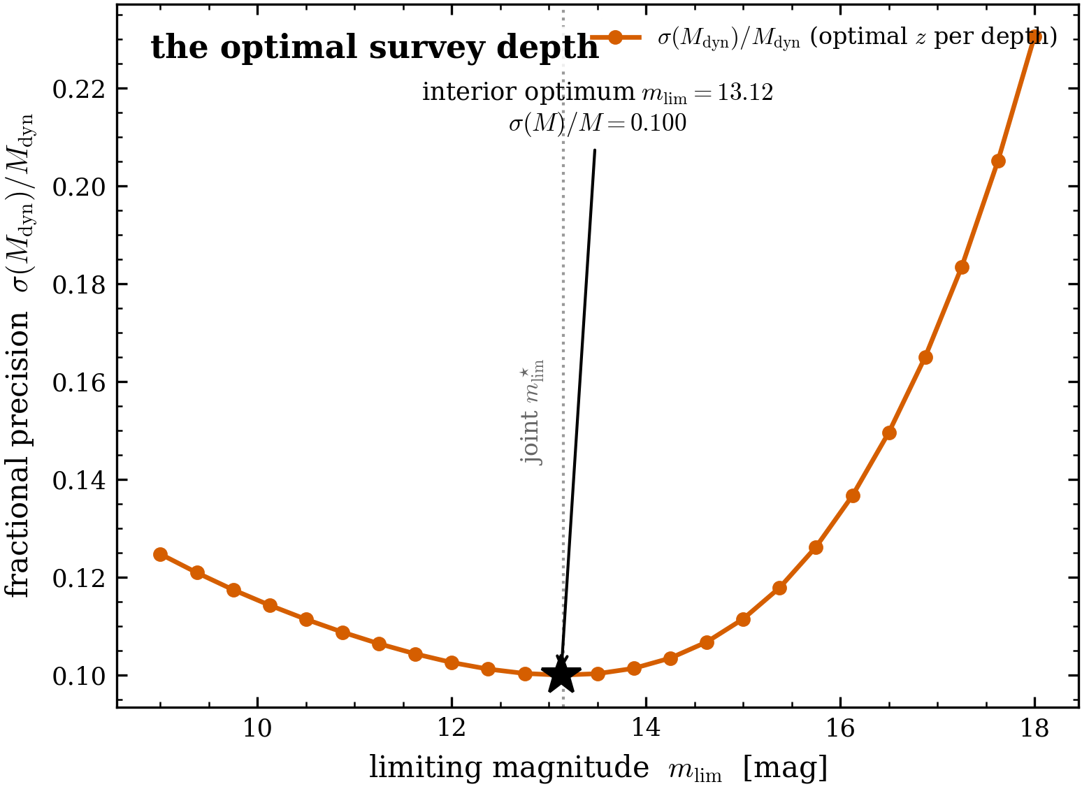
has an interior minimum in survey depth. The fractional precision on the dynamical mass vs the limiting magnitude , at the best allocation for each depth ( kpc, ). The curve falls from a too-shallow survey, bottoms out at near , and rises again toward a too-deep one. The minimum is interior — depth is a real trade-off, not a “more is better” knob.
The mechanism: supply versus noise
Why an interior optimum, with no cost model and no money changing hands? Because depth pulls two levers in opposite directions, and the Fisher information on is their product.
Supply rises with depth. The number of tracer stars depth makes available is the Chabrier IMF integrated above the falling mass floor, summed over the radial bins. Across that available pool climbs steeply, from to stars — and it rises fastest in the star-starved outskirts, exactly where the mass leverage lives.
Noise rises with depth too. The stars depth unlocks are faint, and faint stars are photon-noisy. We model the per-star measurement error with a photon-noise-like scaling (below), so the IMF-weighted effective error climbs as the survey admits ever-fainter tracers — in the RV channel, from to km/s across the same sweep.
Each extra magnitude buys you more tracers but noisier ones. The Fisher information per unit budget — supply divided by noise-variance — therefore peaks in between, and that peak is the optimal depth.
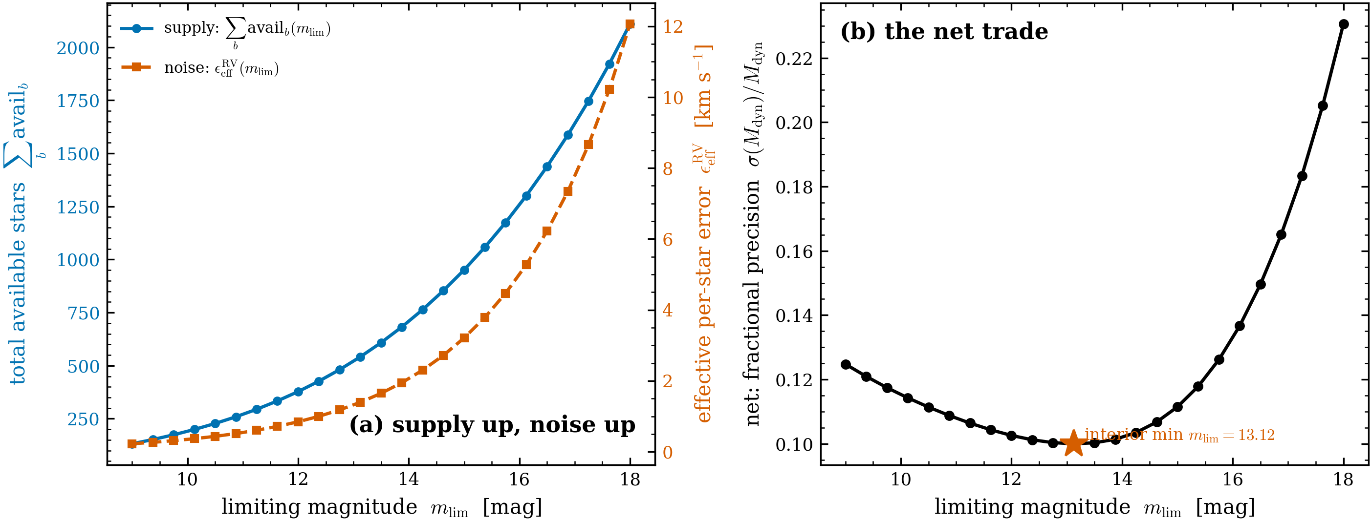
The two competing trends that produce the optimum. Left: the available tracer count (IMF integrated above the mass floor) rises monotonically with depth. Centre: the IMF-weighted per-star effective error rises with depth as fainter, noisier stars enter. Right: their combination — the information per unit budget — peaks at an interior depth, the same as has an interior minimum in survey depth. The fractional precision on the dynamical mass vs the limiting magnitude , at the best allocation for each depth ( kpc, ). The curve falls from a too-shallow survey, bottoms out at near , and rises again toward a too-deep one. The minimum is interior — depth is a real trade-off, not a “more is better” knob.. Supply and noise pull in opposite directions; the optimum is where they balance.
The allocation: weigh the cluster in the outskirts
At the optimal depth, where does the budget go? Almost entirely outside the core. Of the optimal allocation, only of stars sit inside the core radius — go to the outskirts, and within the kinematic channels the radial proper motion dominates while the tangential PM is driven to nearly zero.
That allocation is not arbitrary — it is the mass leverage and the anisotropy talking at once. The dynamical mass is best constrained by the dispersion in the outskirts, where the enclosed-mass profile is flattening toward the total . And the Osipkov–Merritt anisotropy suppresses the tangential dispersion exactly there ( as ), so a tangential-PM star in the outskirts carries little signal — the optimiser correctly spends almost nothing on it.
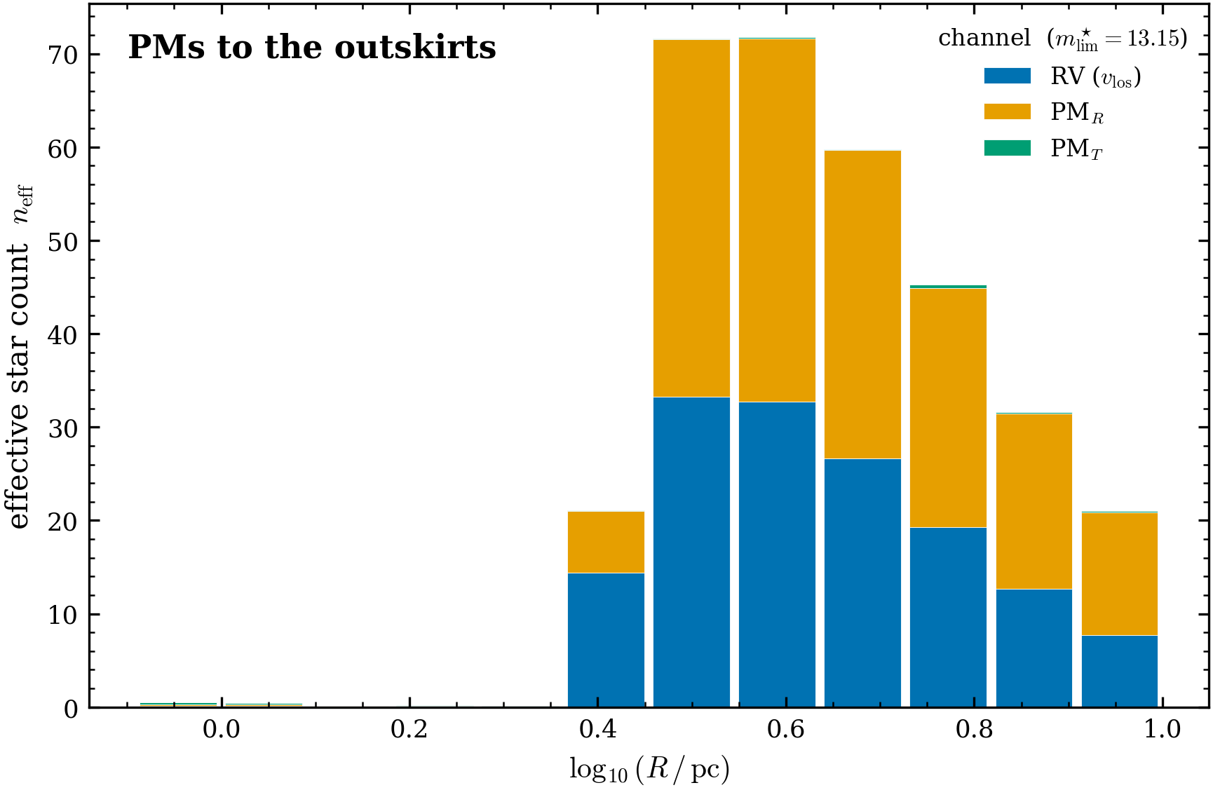
The optimal-depth allocation concentrates in the outskirts. Effective star count per (projected-radius bin × channel) at the joint optimum. The budget piles into the outer bins ( outside the core), with the radial-PM channel carrying the load and the tangential PM near-empty — the outskirts weigh the cluster, and OM anisotropy makes the tangential channel barren there.
The frontier: precision versus budget at the optimal depth
Fix the depth at its optimum and vary the budget. The fractional precision on improves as you add stars, then flattens against the finite supply — once your budget approaches the number of stars the depth actually makes available, more budget cannot help, because there are no more bright-enough stars to measure. At the demo’s the optimal-depth design reaches .
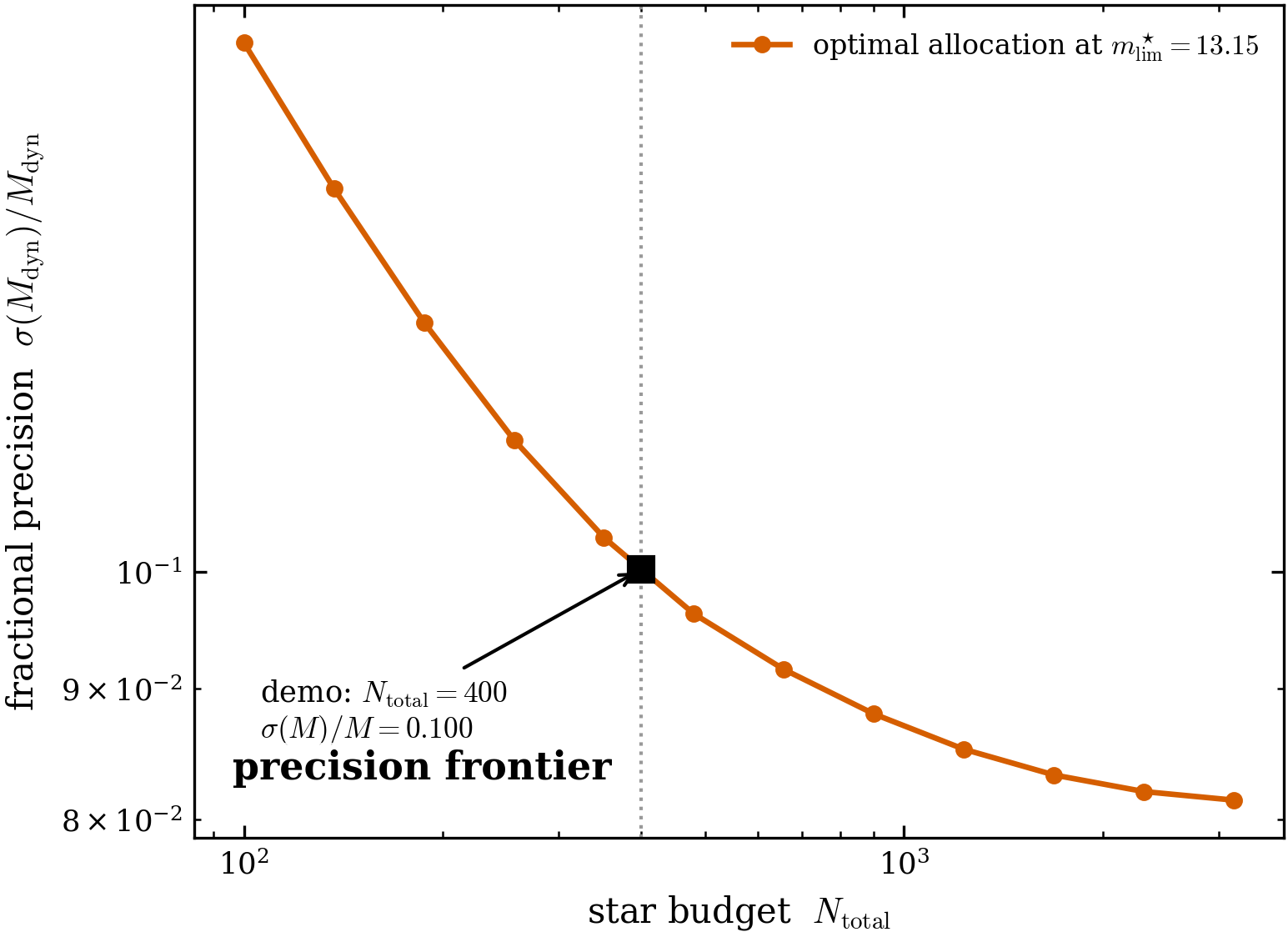
The dynamical-mass frontier at the optimal depth. vs the star budget , evaluated at the optimal . Precision improves with budget but flattens as the budget approaches the depth’s supply ceiling — a real, supply-limited frontier, not an idealised line. The demo point sits at , .
Validating a pre-data calculation: the magnitude-selected calibration
The depth Fisher is a promise about a survey you have not run yet — it deserves the same check as the anisotropy example, but harder: now the mock must respect the magnitude selection itself. We draw a Monte-Carlo ensemble of mock catalogues in which masses are sampled from the Chabrier IMF, only stars with are kept, and each surviving star is given the magnitude-dependent error . We bin, fit by maximum a posteriori, and compare the realised to the Fisher prediction .
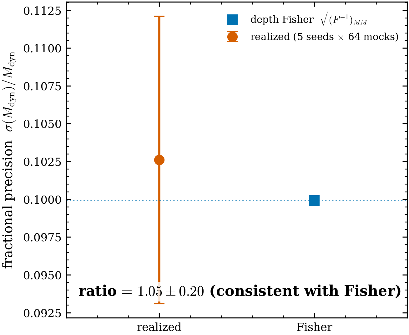
A magnitude-selected mock ensemble confirms the depth Fisher. Realised (from MAP fits to mocks drawn under the same magnitude selection the design assumed) against the Fisher prediction, across the optimal designs. The realised values track the prediction to within (variance ratio –1.05, consistent with 1.0, no significant bias). The depth-dependent selection physics in the Fisher is trustworthy.
Assumptions & approximations
Every modelling choice below is a deliberate simplification with a reason. This is a pedagogical depth knob, not a survey exposure-time calculator — the headline is the shape of the information-versus-depth trade and that an interior optimum exists, both of which are robust to the simplifications. Each choice gets its rationale and the evidence that it is safe here.
1. Bolometric magnitudes (no band, no bolometric correction, no extinction)
We use bolometric magnitudes throughout: with from the ZAMS relation, and no per-band magnitude, no bolometric correction, no interstellar extinction.
Why this is OK here. The headline is the shape of the information-versus-depth curve and the existence of an interior optimum — both set by two band-independent ingredients: the IMF × ZAMS supply (how many stars sit above a given mass floor) and the photon-noise scaling (how error grows with apparent faintness). A real photometric band shifts the mass floor and the error normalisation, but to first order it does not change whether supply-versus-noise produces an interior peak, nor roughly where. The bolometric choice keeps the demo’s physics legible without a colour model getting in the way.
2. Photon-noise error model 
Per-star measurement error scales as , anchored so a reference-magnitude star () has the fiducial error ( km/s, km/s at kpc).
Why this is OK here. The exponent 0.2 per magnitude is the photon-counting scaling: one magnitude fainter is a factor less flux, hence the error. That power law is the correct first-order faint-end behaviour of any photon-limited measurement, which is what sets the rising-noise arm of the trade. It is not a real survey exposure-time calculator — there is no sky background, no detector read noise, no saturation at the bright end, no wavelength dependence. We say so plainly: the scaling captures the trend that drives the optimum, anchored to a bright reference star, and nothing finer.
3. Availability soft-cap 
The design proposes stars per cell, but a cell can only deliver as many stars as actually exist there. We enforce this with a smooth cap, .
Why this is OK here. A finite bright-star supply is real physics — you cannot observe the 50th-brightest star in a bin that contains only 30 — and the optimiser needs to feel it to find an interior depth (without a supply limit, “go shallow and pile every star into the few bright outskirts cells” would be unbeatable). The is the differentiable realisation: for it is (the supply is irrelevant, you take what you ask for), and for it saturates at (you have exhausted the cell). It is a soft constraint chosen for smooth gradients, not a sharp , so the AD-vs-FD gate (below) stays clean.
4. is per-channel global; availability is per-bin
The effective error is one number per channel (an IMF-weighted RMS over the detectable masses), while the availability weight is per radial bin.
Why this is OK here. All stars in the cluster share a single distance . So the mapping from mass to apparent magnitude — and hence the magnitude-dependent error — is the same function of mass everywhere in the cluster; the IMF-weighted error distribution does not depend on which radial bin a star sits in. That makes a per-channel global exact for a single-distance cluster, not an approximation. What does vary with radius is how many stars there are to detect — the projected density falls outward — so availability is correctly carried per bin. The geometry (one distance) is what cleanly factorises error-per-mass (global) from supply (radial).
5. Single-population, mass-follows-light
Every star traces the same potential, so the predicted dispersions are a property of the cluster’s mass distribution — independent of .
Why this is OK here, and why it is the key technical point. Because does not depend on depth, the additive backbone Equation survives untouched: the per-star Jacobian is computed once, and enters only through the cheap, differentiable scalars and . This is what makes optimising over depth affordable — the expensive B&M82 projection is never re-differentiated as the depth changes. The cost is a genuine scope limit: mass segregation and multi-mass kinematics (where lower-mass stars have hotter, more extended orbits, so would depend on which masses you detect) are out of scope. For a single-mass tracer population, mass-follows-light holds exactly.
6. The calibration’s mild design-dependence
The realised/predicted variance ratio is not a single number — it varies across the optimal designs, –1.05.
Why this is honest, not a hidden bias. The spread is consistent with a ratio of 1.0 given the Monte-Carlo error; there is no significant systematic offset in either direction (Important). The leading candidate for the residual scatter is a known subtlety in how the per-channel is formed: it is an IMF-weighted RMS error, whereas the information-optimal combination of heterogeneous per-star errors is an inverse-variance weighting, and the two differ slightly when the error distribution within a channel is broad. We flag this as the most likely source of the mild design-to-design wobble without over-claiming it as a systematic — the calibration’s verdict is that the depth Fisher is trustworthy to , and that is what we report.
The evidence backing these choices
Three quantitative results, all from the gated CLI, are what license the simplifications:
The interior optimum exists and is robust — minimised at –13.3 ( has an interior minimum in survey depth. The fractional precision on the dynamical mass vs the limiting magnitude , at the best allocation for each depth ( kpc, ). The curve falls from a too-shallow survey, bottoms out at near , and rises again toward a too-deep one. The minimum is interior — depth is a real trade-off, not a “more is better” knob.), beating shallow () and deep (). The shape — the actual claim — is exactly what the band-independent supply-versus-noise argument predicts.
The depth gradient is correct — the joint optimiser differentiates through , and an automatic-vs-finite-difference gate on passes at the level. The smooth supply cap and the smooth mass-floor are what keep that gradient clean.
The Fisher is calibrated — the magnitude-selected Monte-Carlo confirms the realised to (Important), under the same selection the design assumed.
Current scope and planned extensions
How to run
# quick (small calibration ensemble, ~1 min)
env -u VIRTUAL_ENV uv run --no-sync python scripts/demo_oed_dynamical_mass.py

# publication-grade (64-draw calibration, ~minutes) — regenerates the figures here
env -u VIRTUAL_ENV uv run --no-sync python scripts/demo_oed_dynamical_mass.py --full
The CLI is gated (exit 0 only if the interior optimum exists, the AD-vs-FD depth gradient passes, and the magnitude-selected calibration lands within band) and writes a JSON run-record alongside the five figures.
References
The shared Fisher / Cramér–Rao / projection theory and its references are on the OED formalism page. The ZAMS – relation is Tout et al. (1996), documented on the ZAMS validation page; the B&M82 sky projection is Binney & Mamon (1982, MNRAS 200, 361); the Osipkov–Merritt anisotropy law is Merritt (1985). The companion design — where, not how deep — is the anisotropy example, and the anisotropy recovery demo is B6.
- Merritt, D. (1985). Spherical stellar systems with spheroidal velocity distributions. The Astronomical Journal, 90, 1027–1037. 10.1086/113810